


Although Demand Side Management (DSM) of Air Source Heat Pumps (ASHPs) offers various potential advantages, it is unlikely to reduce the carbon dioxide (CO2) emissions associated with their operation in the scenarios considered here.
Domestic heating is responsible for a significant proportion of energy use in many nations with temperate climates. In the UK it accounts for 23% of final energy use, resulting in 13% of CO2 emissions [1], [2]. If the grid supply is decarbonised, these emissions could be reduced by electrifying the heating systems [3], [4]. This could be achieved through the widespread use of heat pumps. The characteristics of ASHPs are considered here as they are likely to receive a larger market share than Ground Source Heat Pumps (GSHPs); although GSHPs achieve higher efficiencies they also require relatively large underground heat collectors [5]. ASHPs operate by taking thermal energy from the outside air and raising its temperature such that it can be used for space heating. Their coefficient of performance (COP) is defined here as the heat delivered by the ASHP system divided by its total electrical power consumption.
DSM involves altering the temporal characteristics of the demand where possible such that loads are shifted in time to better coincide with greater availability of electricity. As such, it has been suggested as an approach to help mitigate some of the challenges associated with using intermittent renewable generation; for example coping with the rate of change of supply and less consistent demands on conventional plant and making the best use of generation which is surplus to requirements [6], [7]. Additionally, the electrical grid is in need of reinforcement if it is to manage the larger loads anticipated as a result of widespread adoption of electric vehicles and heating systems.
While investigating the potential for the use of DSM with ASHPs, Kelly and Hawkes [8] observed that a decrease in their performance is likely. However, the study focussed on predetermined load shifts in the context of the current UK generation grid rather than considering the context of a future generation grid with a high penetration of intermittent renewables. Other studies have considered the potential flexibility of ASHP systems but have not provided quantitative assessment of the effect which such approaches may have on the emissions associated with the units [9], [10]. A field trial has been conducted in which a DSM system was used to alter the operation of ASHPs in order to minimise market imbalances caused by imperfect prediction of wind generation [11]. However, the trial focussed upon the practical implementation of such a system rather than the effect which it may have on the performance of ASHP units. The dispatch of micro combined heat and power units has received more attention with studies based on both field trials (e.g. [12]) and modelling (e.g. [13], [14]) but these have tended to focus on DSM strategies based upon local infrastructure constraints. A wider range of potential effects, including aspects considered in the results presented here have been analysed in a larger thesis by one of the present authors [15].
If the operation of ASHPs can be influenced by a DSM system such that they are encouraged to operate when the Marginal Carbon Emissions Factor (MCEF) of the grid is low and discouraged from operating when it is high then it could be hoped that this would reduce the emissions associated with their operation. This study investigates the potential for this benefit.
In order to investigate the effect that this approach might have, ten scenarios have been modelled. Within each of these ten scenarios, the COP and CO2 emissions associated with the operation of the ASHPs have been simulated under a range of conditions. The ten scenarios consist of five different grid generation mixes, considered both with and without DSM applied to the ASHPs. Each scenario is simulated for a period of four months (120 days), covering the majority of the heating season and the period of the highest electrical consumption. Within each of the ten scenarios, the operation of the ASHP is simulated with 512 permutations of operating conditions, each represented by a dwelling type. These permutations are constructed from four climate locations, four building types, four heating programmes and eight variations on either the level of DSM or the responsiveness of the control system in the cases for which DSM is not used. These are described in the following sections.
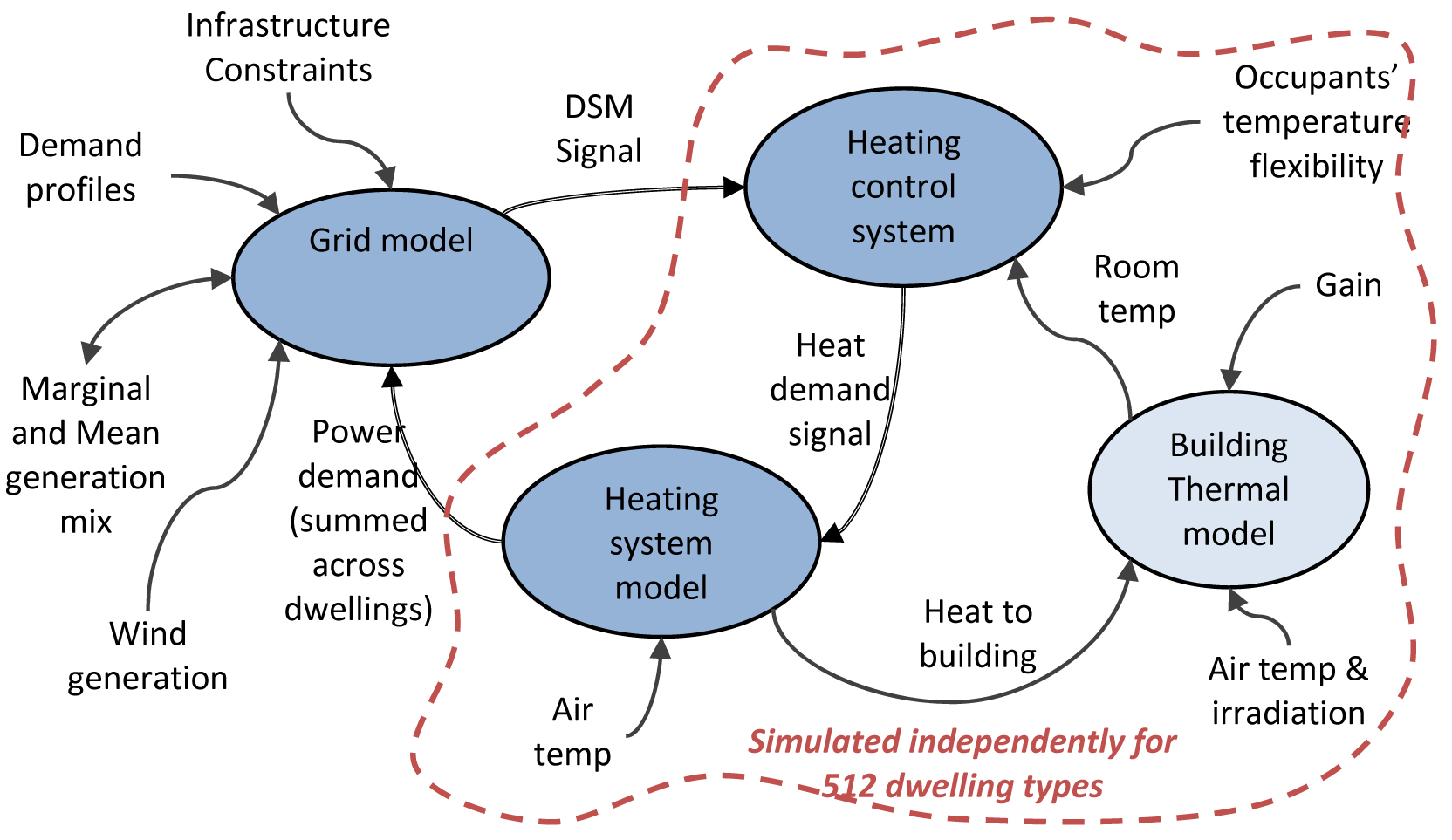
The model is constructed in four interdependent sections; models of the grid, the buildings, the ASHPs and the control systems for them (see Figure 1). Several interactions occur between these sections during each one-minute time-step of the model, as described below. The grid section models the dispatchable generation which is required during each time-step along with the emissions associated with it. The 512 dwelling types are individually simulated, simultaneously, to provide a realistic heating demand profile with adequate diversification. The net electrical demand for the ASHPs in these dwelling types is multiplied by a factor appropriate to the number of actual dwellings using ASHPs in each scenario in order to enable the grid model to calculate the total electrical demand during that time-step.
Overview of interactions between model components
The five grid generation mixes are based on the current (2010) generation mix for the UK, three hypothetical generation mixes based upon the “Transition Pathways” project’s (TP) “Market Rules” scenarios for 2020, 2035 and 2050 (version 2.1) [3], [16] and a fifth generation mix based upon the 2050 mix but assuming that a higher proportion of domestic space heating is met by ASHPs (“2050 +ASHP”). A summary of these generation mixes is given in Table 1.
Description of scenarios (generation totals from [16], [17])
| Scenario: | 2010 | 2020 | 2035 | 2050 | 2050 +ASHP |
|---|---|---|---|---|---|
| Total electrical generation: | 319 TWh | 398 TWh | 488 TWh | 556 TWh | ~581 TWh |
| Generation from nuclear: | 63 TWh | 49 TWh | 89 TWh | 125 TWh | 125 TWh |
| Generation from wind: | 6 TWh | 50 TWh | 112 TWh | 171 TWh | 171 TWh |
| Generation from CCS power plants: | nil | 18 TWh | 169 TWh | 169 TWh | 169 TWh |
| Generation from power plant without CCS: | 245 TWh | 213 TWh | 24 TWh | 1 TWh | See note* |
| Other generation: | 5 TWh | 68 TWh | 95 TWh | 90 TWh | 90 TWh |
| Electric vehicle demand: | nil | 2 TWh | 23 TWh | 38 TWh | 38 TWh |
| Number of dwellings with ASHPs: | 50,000 | 2.56M | 5.12M | 6.14M | 15.4M |
| DSM weighting factor: | 1.7 | 1.8 | 5 | 5 | 5 |
*Because the CCS power plants are used with a high capacity factor, the majority of the increase in demand in the 2050 +ASHP scenario relative to the 2050 scenario is met by conventional CCGT generation. It is possible that this could be resolved by increasing the capacity of the CCS power plant but this has been avoided here so that the results represent a more diverse set of scenarios which remain consistent with the work they are based upon.
Note that each of these scenarios is repeated with and without DSM. These figures (especially for last scenario) are indicative as the exact totals vary depending upon the dynamic nature of the simulation.
For the scenarios involving the present UK grid generation mix, data of historic (2010) electricity generation [17] is used to determine the dispatchable (i.e. combustion-based) generation required during each time-step of the simulations. For the other (future) scenarios based upon the TP generation mixes, a different approach is required. In these cases, it is necessary to determine the generation from each plant type during each time-step. Hypothetical dispatch patterns are constructed by modelling the future demand profiles, subtracting the inflexible generation at each moment from them and then assigning a modified merit-order approach to the dispatch of the combustion based generating plant in order to meet the remaining demand. This is similar to the FESA model [18], [19].
Future demand profiles are based upon the historic profile with some modifications. The profile is adjusted to take into account a simplified electric vehicle charging profile at night-time and the demand from the ASHPs and then scaled to match the total demand appropriate to that scenario. Representative wind generation profiles are generated using an algorithm developed and calibrated by Sturt [20] and subtracted from this profile. The generation from nuclear power plant is scaled from the historic profile to match the scenario total.
Generation from tidal resources is assumed to follow a sinusoidal pattern with periods of 28 days and 12.4 hours. Electrical exports (up to the interconnector capacities) are assumed to take place whenever the resultant demand (i.e. net of wind, nuclear and tidal generation) is less than 3 GW. The remaining demand is then assumed to be met by a mix of Carbon Capture and Storage (CCS) equipped coal-fired power plants and CCS equipped Combined Cycle Gas Turbines (CCGT) in proportion to their share of the total generation in the scenario and up to their generation capacity. When the capacity of the CCS power plant is approached, an increasing proportion of any additional generation demand is supplied by CCGTs. If the capacity of the CCS equipped power plants is exceeded then all additional demand is supplied by conventional CCGTs.
Because this study is considering the potential consequences of a change, it is appropriate to use marginal carbon emissions factors rather than the mean carbon emissions factors. This is achieved by repeating the calculation of the grid generation mix for that time-step, but excluding the demands from the ASHPs. The difference in CO2 emissions between the two cases is then assigned to the operation of the ASHPs, weighted by the power demand of each one.
In each case, the DSM objective is to discourage the consumption of electricity during the times at which it would be generated with a relatively high MCEF and to encourage it when it would be generated with a relatively low MCEF. This is achieved by a DSM signal which varies with time and affects the operation of the ASHPs. Within each time-step, the strength of the DSM signal is determined by iteration between the three darker components shown in Figure 1.
The iteration is as follows. A hypothetical signal is generated, based upon the MCEF of the electricity which would be generated during that time-step and the DSM weighting factor given in Table 1. Different weightings are necessary given the differences between the average MCEF for each scenario. They have been selected such that the DSM signal is neutral when the MCEF is at its average (modal) value for that scenario. The signal is supplied to the heating control systems for the 512 dwelling permutations which each adjust the operation of their ASHPs and feedback the corresponding power demand to the grid. The effect that these amended power demands would have on the MCEF for the grid is then calculated and the iteration repeats. Once the DSM signal is settled upon, the model moves on to the next time-step.
Increasing the DSM signal progressively decreases the temperature at which the control system aims to maintain the inside air of each dwelling, relative to the temperature programme. This temperature adjustment is also proportional to the maximum temperature deviations (both positive and negative) which the occupants of the dwelling find acceptable. Eight possible ranges are simulated (see Table 2). The heating control system applied to each dwelling will not aim for an inside air temperature outside of this range, regardless of the strength of the DSM signal. In practice, it would be problematic to impose a hard limit on ASHP power consumption without regard to the preferences of the occupants. If the occupants feel cold, they are likely to turn on portable electric heaters or other devices which are not subject to DSM, increasing total demand.
Range of temperature deviations acceptable to occupants
| Maximum acceptable positive temperature deviation | Maximum acceptable negative temperature deviation |
|---|---|
| 0 | -1 |
| 0 | -2 |
| 1 | -1 |
| 1 | -2 |
| 1 | -3 |
| 2 | -2 |
| 2 | -3 |
| 3 | -3 |
In order to enable like-for-like comparison between results, the Predicted Mean Vote (PMV [21]) is calculated and the average of negative values found for each dwelling type in each scenario. PMV is a standardised metric for thermal comfort; a value of zero represents continuous adequate thermal comfort whereas a value of -1 represents “slightly cool” conditions and corresponds to an air temperature of around 16 °C for the conditions assumed [22].
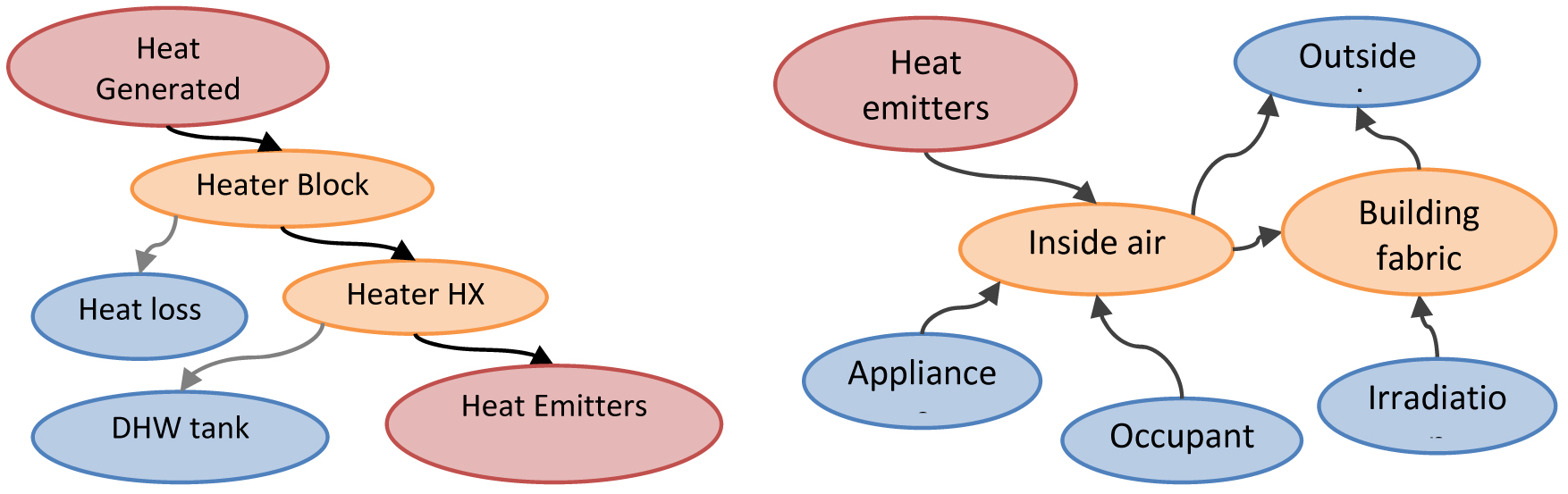
A lumped capacitance approach is taken in order to model each of the 512 dwelling types in each simulation independently. The elements of these models are illustrated in Figure 2. Linear coefficient relationships are assumed for each heat transfer apart from that from the heat emitters which is assumed to exhibit flat-plate buoyancy-driven convective heat transfer [23].
Thermal flows within ASHP model (left) and dwelling model (right)
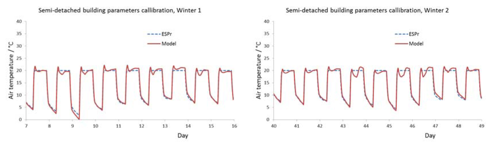
The thermal inertias and heat transfer coefficients for each element of the first three building types were determined by calibrating the temperature profile from each building against that from detailed thermal models simulated using ESP-r by Dr N. Kelly and Dr. J. Hong of ESRU, University of Strathclyde. The properties of these models are based upon representative house types for the UK [2], [24]. The properties of the fourth building type are based upon the first but with improved heat emitter capacities and insulation levels. Although this simplified approach is necessary due to the large number of dwellings simultaneously simulated, good fidelity to the temperature results from the detailed model were achieved (Figure 3).
Air temperature traces from detailed model compared to simplified model
Gains from occupants and appliances are based upon the CREST active occupancy model [25]. Heat emitters are sized such that they require a flow temperature of 45 °C in order to balance heat losses when the buildings are maintained at 21 °C with an external air temperature of -2 °C. Climate data for four locations representing the UK are used (Glasgow, London, Cardiff and Loughborough). Data representative of the present climate (Test Reference Year) and modelled to be representative of the future climate has been provided by the PROMETHEUS project, based upon the UKCIP09 climate model [26].
The steady-state performance of the ASHP which is modelled is taken from performance data provided by [27]. The performance simulated during each time-period is determined by interpolation of the exergy efficiency at the nearest test conditions. A simple thermal model of the unit is also used in order to determine the relevant flow temperature and to account for thermal lags in the system (Figure 2). This is similar to the approach taken elsewhere [28]–[30]. The values of the thermal inertias are based upon the physical characteristics of the heat exchangers (i.e. mass and material) rather than empirically derived temperature plots but produce temperature profiles which are consistent with the range of responsivenesses which are reported. The values of the heat transfer coefficients are calculated from the steady-state temperature drop across the heat exchanger of a similar unit [31].
A proportional controller is employed to determine the heat generated by the ASHP during each time period. The heat generated is proportional to the difference in temperature between the air inside the dwelling and the temperature programme at that moment (adjusted by the DSM signal as explained above). Four temperature programmes are used in order to increase the diversity of the demands and to investigate any difference in the way in which the DSM signal might affect them.
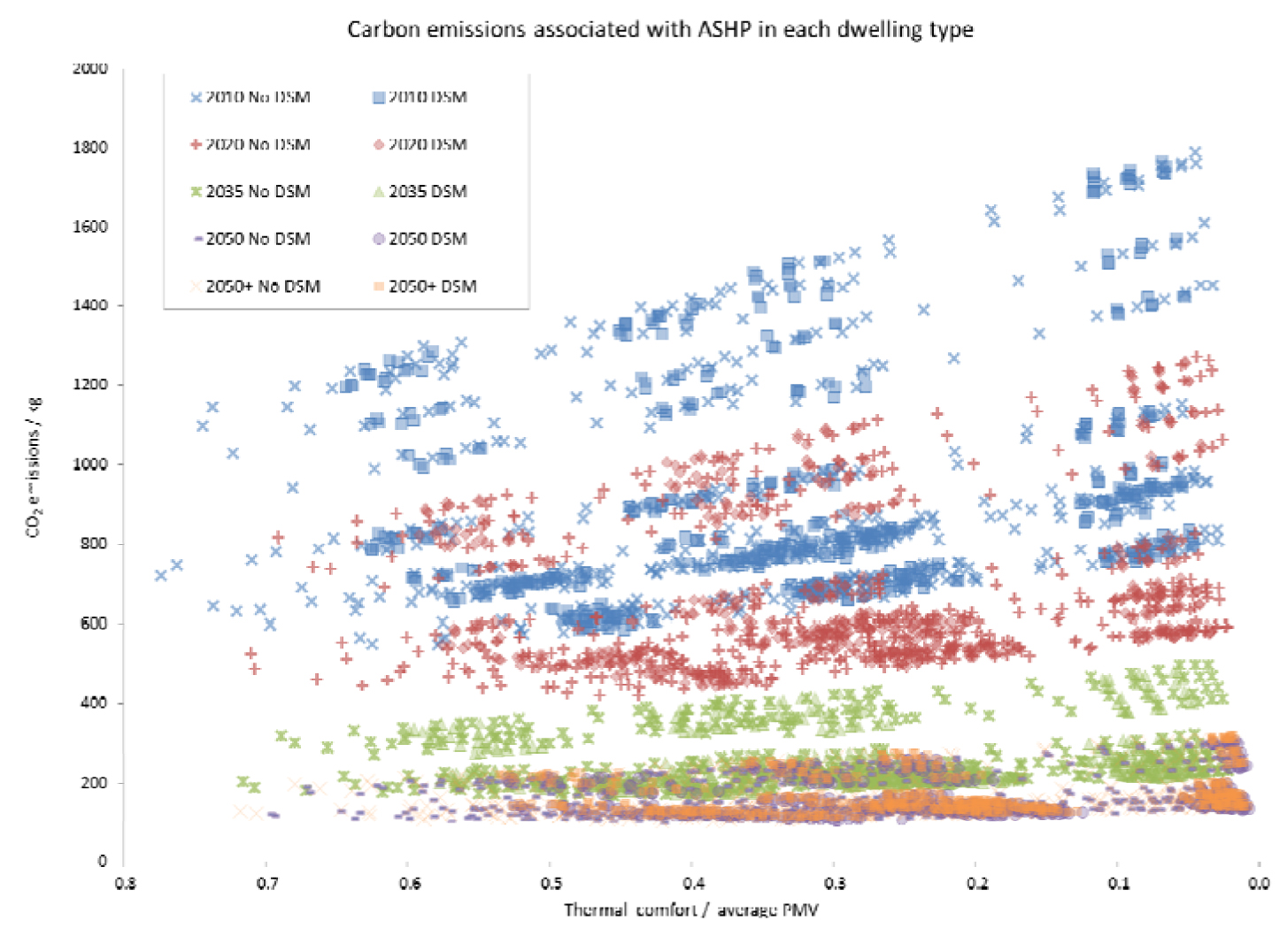
An overview of the CO2 emissions associated with each of the ASHPs is given in Figure 4. Clearly, there is a considerable range of results with both the thermal comfort and CO2 emissions varying widely. The broadly left to right, linear groups within each scenario relate to the groups of scenarios differentiated by the building specification and climate. The variation within each of these groups of results (i.e. with wide variation in thermal comfort but relatively limited variation in CO2 emissions) relates to the different temperature profiles, control system responsiveness and level of DSM in each permutation. Note that the results relate to the 120 day periods simulated, not to an entire year.
CO2 emissions associated with each permutation and scenario
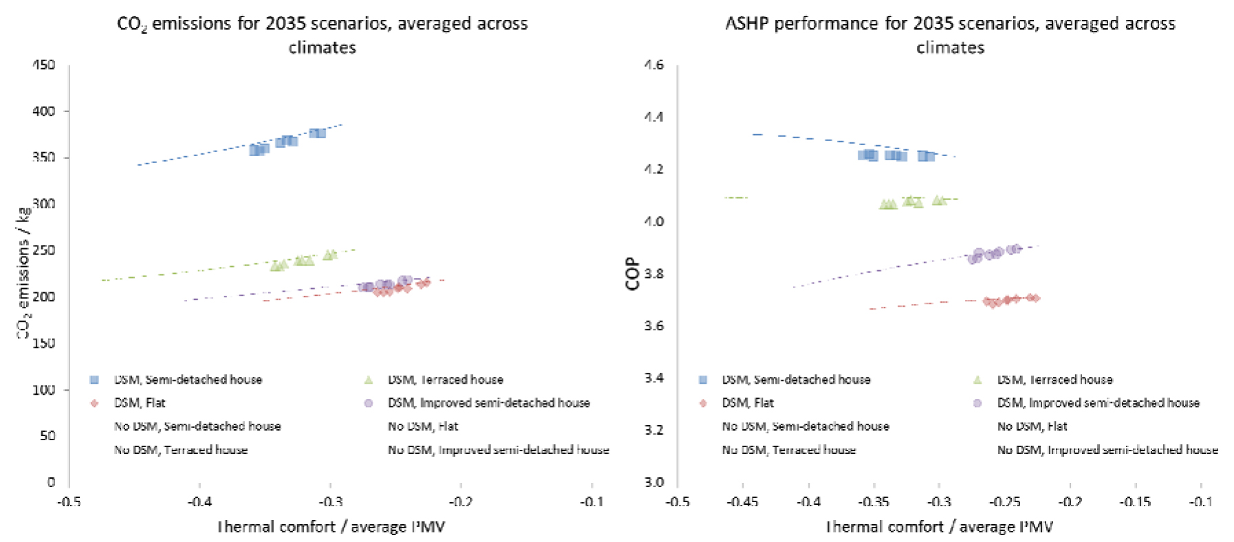
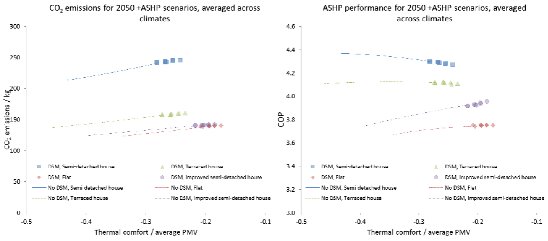
The effect of the different control systems on the performance of the ASHPs can be more clearly observed by taking the mean results across the four climates and by considering the grid scenarios separately. This is shown in Figure 5 and Figure 6 for the 2035 and 2050 +ASHP scenarios. The results for the scenarios in which DSM is not used are presented as plots rather than individual data as their range reflects a continuous set of possibilities which is only dependent upon the control system responsiveness used. In each scenario, the different building types have a large effect on the CO2 emissions associated with them but a similar trend in emissions with thermal comfort.
ASHP performance in 2035 scenarios (CO2 emissions left, COP right)
ASHP performance in 2050 +ASHP scenarios (CO2 emissions left, COP right)
In the 2035 scenarios, a slight reduction in CO2 emissions is observed (approximately 3%) for the cases in which DSM is used compared to the cases in which it isn’t at the same level of thermal comfort. This underwhelming result can be partially explained by reference to the COP achieved by the ASHP in each scenario. In the cases in which DSM is used, a slight reduction in COP occurs which partially offsets the advantage of preferentially operating at times when the marginal CO2 emissions factor is lower. The reduction in COP is due to the increase in average flow temperature which is required in order to deliver heat more rapidly at certain times in scenarios which involved DSM.
The effect of the DSM is different in the 2050 +ASHP scenario. Rather than decreasing the thermal comfort, the DSM signal actually increases it. The CO2 emissions slightly increase with this increase of thermal comfort but not at the same rate as they do with the non-DSM control system.
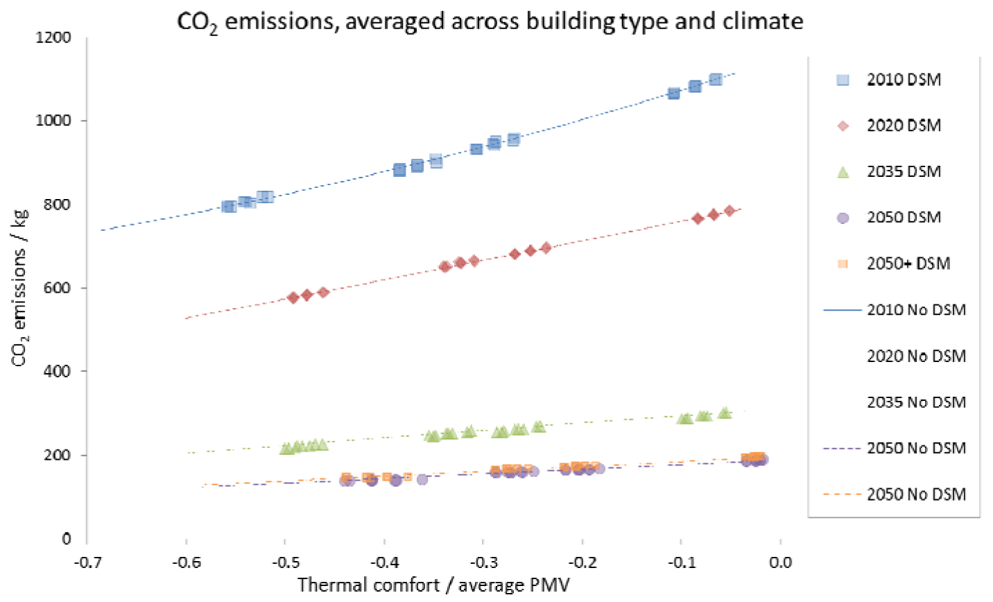
By averaging across building types as well as climate, all of the results can be compared (Figure 7). The four groupings of data which can be observed for each scenario relate to the four temperature programmes used. In the 2010 to 2035 scenarios, the three sets of indistinguishable data points within each of these groups relate to the three values of maximum temperature decrease which the occupants of a dwelling will tolerate (-1 °C, -2 °C or -3 °C). In the 2050 scenarios, the four sets within each group relate to the four values of the maximum temperature increase which are available to the DSM system (+0 °C, +1 °C, +2 °C or 3 °C).
CO2 emissions averaged across building type and climate
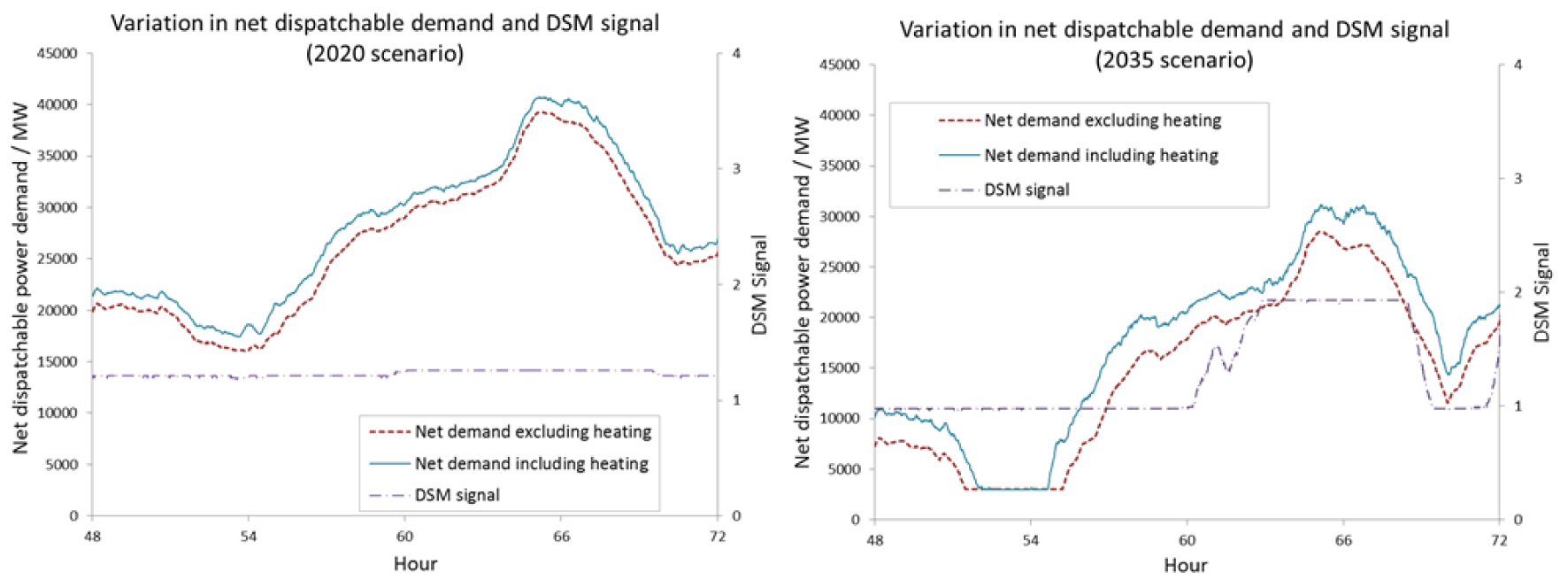
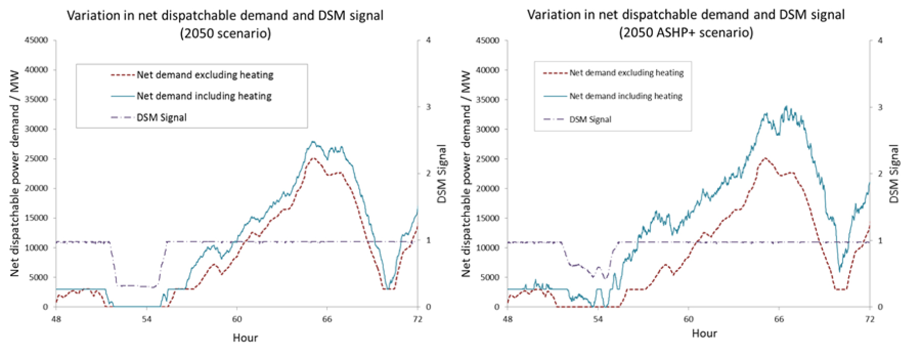
This helps to explain the relatively insignificant effect which the use of DSM is observed to achieve; the changes in the marginal emissions factor for the grid are quite limited in each scenario. This is further illustrated by the demand profiles illustrated in Figure 8 and Figure 9. These show the profile of net dispatchable demand after wind, nuclear and other non-dispatchable generation have been accounted for.
Demand profile for 24 hours in 2020 (left) and 2035 (right)
Demand profile for 24 hours in 2050 (left) and in 2050 with additional ASHPs (right)
In the 2020 scenario, the DSM signal shows little fluctuation as the MCEF remains fairly constant across the 24 h period, most dispatchable generation is from CCGTs without CCS.
In the 2035 scenario, there is significantly more CCS equipped plant and so the main effect on the DSM signal is an increase (i.e. discouraging ASHP use) when dispatchable demand is high and a greater proportion of additional demand would come from CCGTs without CCS (e.g. hours 60 to 69). In the plots for both 2020 and 2035, there is no point at which the MCEF drops below the level of CCS plant (i.e. dispatchable plant is always required) and so the DSM does not encourage higher temperatures (resulting in the three sets of data in each grouping observed in Figure 7). The 2035 scenarios show the greatest variation in the MCEF of electricity and is subsequently the only scenario in which some reduction in emissions is achieved by the DSM (Figure 5 and Figure 7).
Conversely, almost all dispatchable generation is met by CCS equipped plant in the 2050 scenarios. The DSM signal therefore rarely discourages consumption. However, there are periods (e.g. hours 52 to 56) when there is no dispatchable generation demand (and so renewable generation will be constrained) and so the DSM signal encourages consumption with higher temperatures. This explains the relatively higher (i.e. less negative) groupings of PMV values relating to these scenarios in Figure 6 and Figure 7; the DSM rarely causes a decrease in the temperature within dwellings in these scenarios. Although the temperatures within the dwellings are increased at times using the low MCEF electricity, this does not lead to a significant net reduction in electricity demand at other times. This finding suggests that alternative storage methods such as phase change materials or thermal storage which can be bypassed during warmer periods may decrease the CO2 emissions resulting in these scenarios.
Although the DSM signal had a limited net effect on emissions in these scenarios, it did decrease the COP of the ASHP relative to the equivalent conditions without DSM, (see Figure 10).
Effect of DSM signal on COP of ASHP
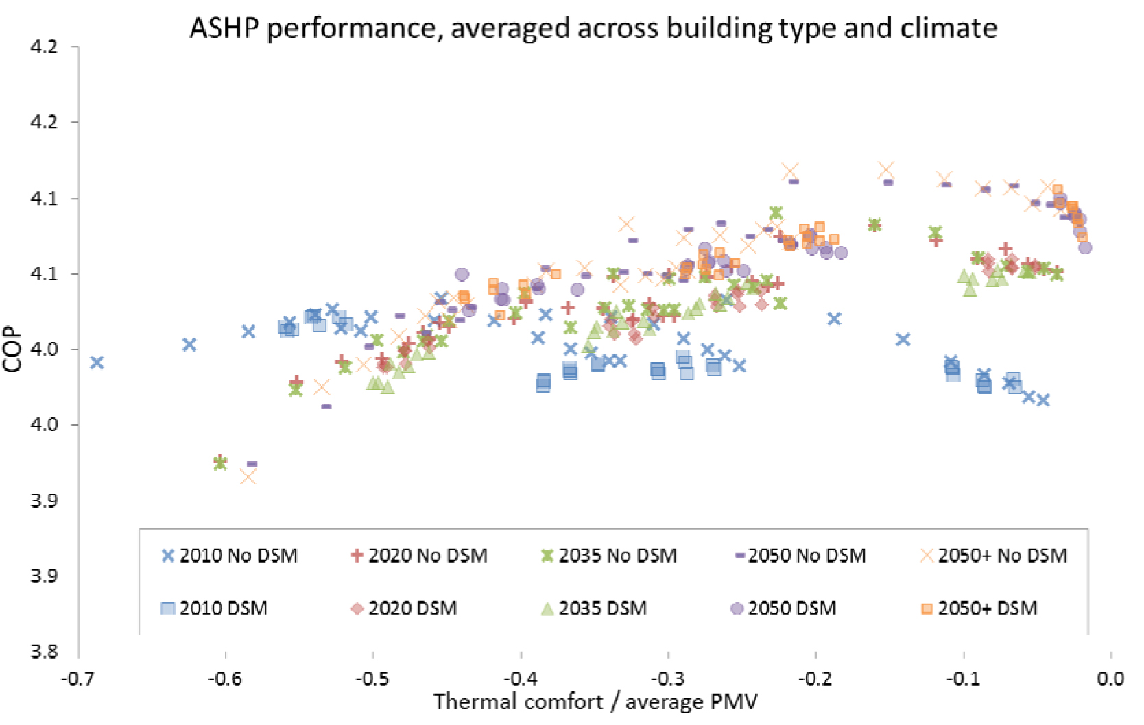
This is a similar effect to that noted elsewhere [8] and suggests that DSM schemes which might use a stronger signal or not give consideration to the MCEF of the electricity could increase the CO2 emissions associated with the use of the ASHPs. This potential effect should be considered when evaluating the relative merits of such systems.
A model has been constructed to enable investigation of performance and emissions associated with ASHPs when DSM is used. This has been used to investigate the potential reduction in CO2 emissions which could be achieved by a DSM signal that encourages consumption when the MCEF is low and discourages it when the MCEF is high. In the scenarios investigated, the emissions reduction which could be achieved was found to be small. A reduction of around 3% was observed in scenarios based around 2035 but in other scenarios the reduction was insignificant. In the scenarios with high wind generation (2050), the DSM scheme considered here tends to improve thermal comfort (with minimal increases in emissions) rather than achieving a decrease in emissions. Other schemes may also achieve reductions but given the negative impact which the DSM signal has on the COP of the ASHPs, the possibility of increased emissions should also be recognised.
Air Source Heat Pump.
Combined Cycle Gas Turbine.
Carbon Capture and Storage.
Carbon dioxide.
Coefficient of Performance, the quotient of heat delivered and power consumed.
Demand Side Management.
Ground Source Heat Pump.
Marginal Carbon Emissions Factor, the CO2 emitted per additional unit of electricity generated.
Predicted Mean Vote, a measure of thermal comfort.
Transition Pathways, the project providing the hypothetical future grid mixes.
This work was supported by various research grants awarded by the UK Research Councils’ Energy Programme (RCEP), and Engineering and Physical Sciences Research Council (EPSRC) as part of the SUPERGEN Highly Distributed Energy Futures (HiDEF) consortium [Grant number EP/G031681/1; for which Prof. Hammond was a Co-Investigator]. The consortium involves a number of academic and industrial partners, coordinated by Prof. Graeme Burt and Prof. David Infield; both with the Institute for Energy and Environment at the University of Strathclyde. Prof. Hammond is also jointly leading a large consortium of university partners (jointly with Prof. Peter Pearson, Director of the Low Carbon Research Institute) funded via the strategic partnership between e.on UK and the RCEP to study the role of electricity within the context of ‘Transition Pathways to a Low Carbon Economy’ [Grants EP/F022832/1 and EP/K005316/1; for which Prof. Hammond is the PI and co-leader]. The authors gratefully acknowledge the interchange made possible under these programmes. However, the views expressed here are those of the authors alone, and do not necessarily reflect the views of the collaborators or the policies of the funding bodies.
In particular, the help of Nick Kelly and Jun Hong from ESRU, University of Strathclyde and of Ian Richardson and Murray Thompson of CREST, Loughborough University in calibrating models is gratefully acknowledged. Authors’ names appear alphabetically.
- , , The UK Low Carbon Transition Plan, 2009
- , , Great Britain’s housing energy fact file, 2011
- ,
“Developing transition pathways for a low carbon electricity system in the UK,” in ,Technological Forecasting and Social Change , Vol. 77 (8), :1203-12132008, https://doi.org/10.1016/j.techfore.2010.04.002 - , , Home Truths: A low-carbon strategy to reduce UK housing emissions by 80% by 2050, 2007
- , , Heat Pumps, Technology and Environmental Impact, 2005
- , “Impact of intermittency: How wind variability could change the shape of the British and Irish electricity markets,”, 2009
- ,
“Demand side management: Benefits and challenges,” ,Energy Policy , Vol. 36 (12), :4419-4426Dec. 2008, https://doi.org/10.1016/j.enpol.2008.09.030 - ,
“Load management of heat pumps using phase change heat storage,” in ,Proceedings of 3rd International Conference in Microgeneration and Related Technologies in Buildings: Microgen 3, Naples, Italy, 15 - 17th April 2013 , 2013 - ,
“Assessing heat pumps as flexible load,” ,Proceedings of the Institution of Mechanical Engineers, Part A: Journal of Power and Energy , Sep. 2012 - ,
“Heat pumps and energy storage – The challenges of implementation,” ,Applied Energy , Vol. 89 (1), :37-44Jan. 2012, https://doi.org/10.1016/j.apenergy.2010.12.028 - ,
“Wind Turbine and Heat Pumps – Balancing wind power fluctuations using flexible demand,” in ,Sixth International Workshop on Large-Scale Integration of Wind Power and Transmission Networks from Offshore Wind Farms , 1-92007 - ,
“Virtual power plant field experiment using 10 micro-CHP units at consumer premises,” in ,CIRED Seminar 2008: SmartGrids for Distribution, Frankfurt, 23 - 24 June 2008 , (86), 2008 - ,
“Controlling micro-CHP systems to modulate electrical load profiles,” ,Energy , Vol. 32 (7), :1093-1103Jul. 2007, https://doi.org/10.1016/j.energy.2006.07.018 - ,
“Performance implications of heat pumps and micro-cogenerators participating in demand side management,” in ,Proceedings of 3rd International Conference in Microgeneration and Related Technologies in Buildings: Microgen 3, Naples, Italy, 15 - 17th April 2013 , 2013 - , , Thermodynamic Analysis of Air Source Heat Pumps & Micro Combined Heat & Power Units Participating in a Distributed Energy Future, 2013
- ,
“Transition pathways for a UK low carbon electricity future,” ,Energy Policy , 1-15Jun. 2012 - ,
Elexon, “Balancing Mechanism Reports,” , 2012, (Online). Available: http://www.bmreports.com/. (Accessed: 10-Jun-2012) - ,
“The evolution of electricity demand and the role for demand side participation, in buildings and transport,” ,Energy Policy , Vol. 52 , :85-102Sep. 2012, https://doi.org/10.1016/j.enpol.2012.08.040 - ,
“Modelling generation and infrastructure requirements for transition pathways,” ,Energy Policy , 1-16May 2012 - ,
“Time series modelling of power output for large-scale wind fleets,” ,Wind energy , Vol. 14 (8), :953-9662011, https://doi.org/10.1002/we.459 - ,
“Assessment of man’s thermal comfort in practice.,” ,British journal of industrial medicine , Vol. 30 (4), :313-24Oct. 1973 - , , Ergonomics of the thermal environment — Analytical determination and interpretation of thermal comfort using calculation of the PMV and PPD indices and local thermal comfort criteria, 2005
- , , Fundamentals of heat and mass transfer, 1985
- ,
“Identifying characteristic building types for use in the modelling of highly distributed power systems performance.” , 2010 - ,
“A high-resolution domestic building occupancy model for energy demand simulations,” ,Energy and Buildings , Vol. 40 (8), :1560-15662008, https://doi.org/10.1016/j.enbuild.2008.02.006 - ,
“On the creation of future probabilistic design weather years from UKCP09,” ,Building Services Engineering Research and Technology , Vol. 32 (2), :127-142Oct. 2010, https://doi.org/10.1177/0143624410379934 - , Warmepumpen-Testzentrum, Test results of air to water heat pumps based on EN 14511:2011, 2013
- ,
“Analysis of retrofit air source heat pump performance: Results from detailed simulations and comparison to field trial data,” ,Energy and Buildings , Vol. 43 (1), :239-245Jan. 2011, https://doi.org/10.1016/j.enbuild.2010.09.018 - , , Specifications for Modelling Fuel Cell and Combustion-Based Residential Cogeneration Devices within Whole-Building Simulation Programs. A Report of Subtask B of FC+COGEN-SIM The Simulation of Building-Integrated Fuel Cell and Other Cogeneration Systems. A, 2007
- ,
“Thermodynamic efficiency of low-carbon domestic heating systems: heat pumps and micro-cogeneration,” ,Proceedings of the Institution of Mechanical Engineers, Part A: Journal of Power and Energy , Vol. 227 (1), :18-29Oct. 2012, https://doi.org/10.1177/0957650912466011 - , Mitsubishi Electric Europe, Service manual, 2008