


The EU’s climate neutrality goals include energy efficiency in the energy sector, and the Natural Gas (NG) sector, despite being based on the cleanest fossil fuel and having the longest survival horizon, must still ensure an increase in energy efficiency and progressive decarbonisation. There are several areas to act on for the decarbonisation of the gas transport infrastructure, to name a few: decarbonisation of the gas carrier through injection of green gases such as biomethane [1] or hydrogen [2], [3], reduction of fugitive emissions into the atmosphere [4] and finally reduction or elimination of gas burned in pre-heating systems in City Gate Stations (CGS) [5]. The gas infrastructure can be divided into high-pressure transport networks and medium and low-pressure networks for distribution to end-users. The transition from the high-pressure network to the low-pressure network is managed by CGS, and this is where pressure reduction by throttling takes place. It is a dissipative process requiring the insertion of gas-fired preheaters to prevent the gas from cooling too much downstream of the lamination valve and allowing hydrates to form. Furthermore, low gas temperatures can reduce the operational safety of control valves. The pre-heating station generally retains some of the gas passing through the CGS and burns it in boilers to heat a pre-heating water circuit [6]. Therefore, it is vital to investigate possible solutions to decarbonise this energy-intensive process.
NG pre-heating efficiency and energy recovery have already been studied in several scientific papers; academic studies generally deepen two approaches: energy recovery in the gas through expanders that exploit the residual pressure drop to produce electricity or systems for reducing or diminishing the energy cost of pre-heating the gas.
Farzaneh-Gord et al. propose a heat production system as a partial replacement for the traditional boiler consisting of a solar collector coupled to a tank, applied to a CGS placed in Akand. The authors find the optimal number of collectors and storage tank capacity based on the technical-economic analysis; as the number of collectors increases, the fuel cost decreases, but the capital cost increases [7].
Farzaneh-Gord et al. then propose a new system to eliminate the fuel consumption of CGSs, using a ground-coupled vertical heat pump. The system’s performance is studied under two different climatic conditions in Iran and two different NG compositions. Results show that the system can fully eliminate pre-heating gas consumption by more than 65% and reduce CO2 emissions by up to 79%. The discounted payback period is computed to be around two years [8].
Borelli et al. investigate the integration of a CGS with low-temperature thermal energy sources employing a two-stage expansion system. The risk of NG hydrate formation was evaluated for several Operating Conditions (OCs) with a transient model. The energy efficiency of the cabinets with low and high-temperature configurations is compared. Results highlight that the expansion could achieve better energy performance and be integrated with low-enthalpy heat sources [9]. The same authors investigate and propose Key Performance Indicators (KPIs) for energy recovery in CGS, considering a theoretical reference process in which Joule-Thompson expansion and emission reduction indicators occur. Results showed that the proposed KPIs proved to be a useful, simple, and easily interpretable tool for managing the design development of heat recovery systems at CGS [10].
Englart et al. propose using renewable energy sources in CGS Polish gas pre-heating to reduce thermal energy consumption, analysing various combinations with a conventional heat pump, absorption, and ground heat exchanger. Results highlight that applying a gas heat pump to replace the traditional gas boiler could reduce gas consumption by up to 27−42% for the case study considered. Extending the gas pre-heating system with an additional ground heat exchanger, used as a heat source for the heat pump, could lead to greater energy savings in gas consumption of between 30 and 44% [11].
In a study for the following year, the authors focus on renewable energy source (RES)-based electrical technologies, such as air source and ground source heat pumps, coupled with air-to-ground heat exchangers and horizontal and vertical heat exchangers. The pre-heating estimation model is improved from previous work by considering the gas composition to estimate the basic properties of the fuel chemical compounds. Analyses were performed for three climate types (from cold to hot) and the two operating modes. Results show that the electric pre-heating solution with a RES system can save more than 50% of the primary energy, reducing greenhouse gas emissions [12].
Danieli et al. [13] study several kinds of mechanical expanders combined with different pre-heating devices based on gas boilers, cogeneration engines or heat pumps to identify the best combination by evaluating the combination of maximum net present value and minimum payback period applied to Pressure Reduction Stations (PRS). Results show that small-size volumetric expanders with low expansion ratios coupled with gas-fired preheaters have the highest potential for large-scale deployment of energy recovery from PRSs with a maximum recovery percentage of about 15% of the available thermal energy. In the following paper [14], the above authors evaluate a thermal energy recovery system’s economic and technical feasibility analysis based on the Ranque-Hilsch vortex tube. A model of the entire system is included in an optimisation method. A new empirical model of the device is proposed. Finally, a complete set of PRS from the Italian NG grid is chosen as a case study, using the actual operating conditions collected by the DSO of each station. Results point out that the ambient temperature strongly influences the techno-economic feasibility of the proposed device, but 95% of pre-heating costs could be eliminated with a payback time of less than 20 years.
Mohammad Ebrahimi Saryazdi et al. perform a multi-objective optimisation of an NG pre-heating system composed of a turbo-expander supplied by a waste heat recovery device or a boiler unit. The proposed configuration’s total cost and exergy are used as objective functions. Results show that the configuration without the gas boiler unit benefits economic and exergy indicators [15].
Alizadeh et al. study the possibility of improving the energy recovery efficiency in CGS using a heat pipe designed specifically for this purpose. This system is tested with real data from one year of operation of pressure reduction stations. Results indicate that the heat pipe can reduce gas consumption by more than half a million cubic meters a year, preventing 756 tonnes of CO2 from being emitted [16].
In Italy, there are more than 9000 stations for NG pressure reduction and measurement, with pressure drop ratios varying up to 20 and extremely variable power sizes. However, most CGS in Italy process flow rates below 2000 Sm3/h and, as a result, classic turbo expander solutions, considered the most advantageous for energy recovery, may be economically unviable [13].
Some of the limitations of the studies concern estimating pre-heating consumption employing models that are simplified or not always compared with experimental data, or the choice of analysing very complex and specific systems based on expanders or other technologies, not always followed by a detailed analysis of the economic feasibility of the chosen system. If we were to divide a techno-economic analysis into two main parts, most articles studying this topic do not comprehensively examine the two aspects and focus on one at most.
On the contrary, in the first part of this analysis, a thermodynamic calculation model is developed, considering the actual operating conditions of such a plant. In contrast, in the second part, an economic analysis is carried out, which considers all indices and parameters.
The real operating conditions are influenced by manual adjustments of the set point of gas outlet temperature in relation to seasonality, a load curve strongly dependent on the downstream aggregate demand curve, and the gas temperature input conditions. The economic part was addressed by clearly specifying all cost indices and gas energy prices and introducing a relevant aspect such as energy efficiency certificates, the functioning of which was presented to us by working with the industrial partner who provided us with the pre-validation data for the model.
In summary, the work provides an understanding of the effect of all parameters affecting the techno-economic feasibility of such an intervention. It proposes to develop a simplified yet refined and generalisable method to analyse the feasibility of reducing thermal energy consumption in a CGS equipped with RES-based heat pumps.
For this work, a dataset of a CGS located in central Italy is exploited, which, relative to a medium-small operational size, is considered sufficiently representative of many of the CGS present in the Italian scenario.
The following chapter presents the thermodynamic model used to estimate the annual heat load and its validation. Next, the layout of the proposed hybrid system is presented, and finally, the results of the technical and economic analysis of the proposed system are illustrated and analysed. However, the methodology can be generalised to all CGS, knowing the input values explained in the discussion.
A new layout for the NG pre-heating system is proposed based on integrating a RES-based Heat Pump (HP) with the conventional gas-fired Boiler Unit (BU). The system is equipped with an Air Source Heat Pump (ASHP) fed by a Photovoltaic (PV) field, as shown in Figure 1. The various components of the CGS described in the figure will be explained in the following paragraphs.
Natural gas pre-heating hybrid system layout
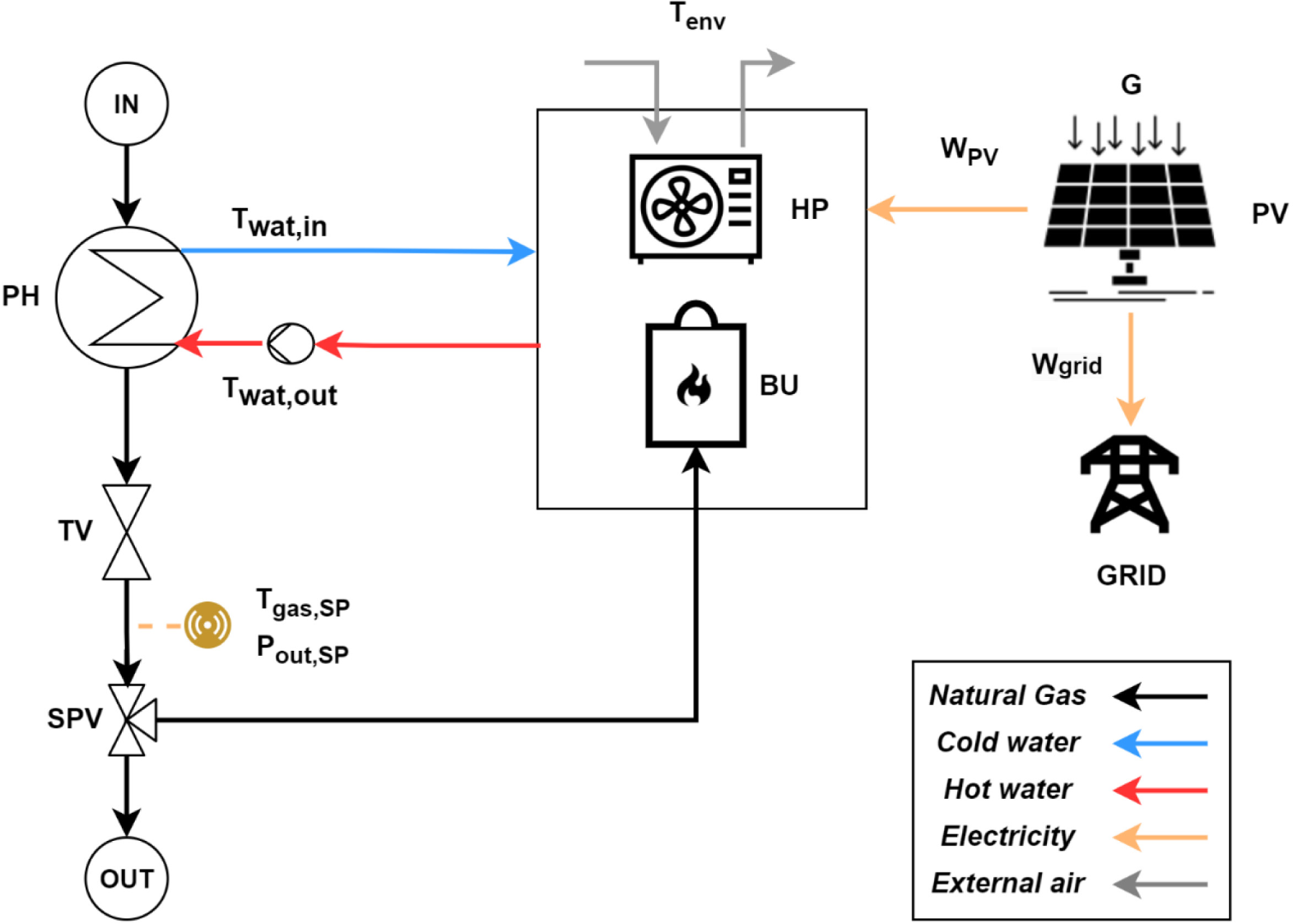
The assumptions underlying the operation of the HP are to utilise the outside air as a thermal reference well and to send water at a temperature of 55 °C to the Preheater (PH) to pre-heat the gas before it enters the Throttling Valve (TV). This assumption is made reasonably to maintain a safety coefficient at the exchanger to avoid flow crossings at any time of the year and, simultaneously, not to penalise the heat pump’s efficiency too much.
The flow rate is not calculated; it is assumed that the system can modulate it with an inverter to the pumps to manage the heat supplied to the gas optimally.
Every timestep Δt, assumed equal to 1 hour, the power balance between the pre-heating power demand of natural gas Wgas, for the given input conditions and output set points, and the heat output that can be supplied by the heat pump WHP,th is calculated.
The heat pump always has priority whenever there is a surplus of renewable thermal energy (i.e., electric power from the PV), all the pre-heating requirements are fulfilled with the heat pump, and the equivalent surplus electricity is sold to the grid. On the other hand, if the heat output supplying the HP is zero or insufficient, the auxiliary boiler comes into action, and the necessary NG flow rate is obtained from the primary flow via the Splitting Valve (SPV).
The control balance of the logic is described by equation (1) where WBU is the boiler power to cover the thermal power deficit Wdef, Wgrid is the electrical power fed into the grid by the photovoltaic surplus Wsurp; the various models of the components of the equation will be described in the following paragraphs.
(1)
The electric power which can be exploited by the ASHP every hour Wel,HP is obtained following a control logic that compares the power output of the solar panels WPV(t) with a “cut-off” threshold ε: when the solar field output is equal or higher to the ε the heat pump is switched on, but when the value of Wel,PV(t) falls below ε the heat pump is switched off.
(2)
The cut-off threshold is obtained by considering the advice given by the DSO and is set to 1 kW to avoid drops in the heat pump’s efficiency below the value of supplied electrical power. The heat output that the heat pump can provide every hour will be given by the product of the available electrical power and the actual coefficient of performance COP(t).
(3)
Every timestep Δt, if the total power balance is higher than 0 (thermal energy deficit), the heat output to be supplied by the auxiliary boiler is calculated according to (4) as the difference between the required heat output and the heat output supplied by the HP calculated with the previous equation.
(4)
The total annual thermal energy supplied by the auxiliary boiler [kWh/year] is given by:
(5)
The total annual thermal energy saved will be the thermal energy supplied by the pump instead of, or together with, the auxiliary boiler.
(6)
When it comes to RES systems based on PV plants, the main parameters to be considered to assess the self-sufficiency level of the system are the SSR (Self Sufficiency Ratio) and SCR (Self Consumption Ratio), generally defined as ratios of amounts of electricity [17].
In this study, since annual demand is thermal, the SSR of the RES system is adjusted to the considered case study and defined as the ratio between the self-consumed thermal energy and the total yearly energy demand (7); these two parameters are obtained from the previous equations.
(7)
On the other hand, the SCR can be expressed as the ratio of self-consumed electric energy and the total yearly energy production.
(8)
Where Eel,sav,y is obtained directly from the Eth,sav,y knowing the actual COP value every timestep according to environmental conditions, EPV,y is the annual PV electric energy output and Egrid,y is the annual electricity sold to the grid.
The thermal power Wgas used by the control logic of equation (1) and required to heat the standard gas flow rate Qst,gas before it enters the throttling valve is given by the equation below:
(9)
Where ρst,gas is the NG density, cp,st is the specific heat capacity, both evaluated according to standard conditions; Δt_gas is the gas temperature increase, and η is the pre-heating system efficiency, equal to 0.9.
The definition of the standard condition is crucial when dealing with the natural gas distribution system in the Italian scenario, which reasons in terms of energy and not in terms of the volume of gas dispatched. Standard cubic meters are defined as the amount of gas contained in one cubic metre at standard conditions of temperature (15 °C) and pressure (101325 Pa, i.e. atmospheric pressure) [3]. Henceforth, all volume or flow rate definitions will be expressed in standard cubic metres (Sm3).
The NG thermodynamic properties are assumed constant and equal to ρst,gas = 0.76252 kg/Sm3 and to cp,st = 2.160 kJ/kg K, according to the annual values given by the Italian Transport System Operator (TSO) [18]. The required gas temperature increase is calculated using (10), where ΔTgas is the sum of the difference between the inlet temperature and the outlet temperature ΔTOI and the temperature decrease due the Joule-Thomson effect.
(10)
(11)
(12)
The temperature decrease due to the Joule-Thomson effect is given by (12), where μJT is the Joule-Thomson coefficient in °C/MPa and ΔPgas is the pressure drop, which is calculated with the following equation:
(13)
Where Pgas,in is the gas inlet pressure and Pgas,out is the value of the gas outlet pressure, which is kept fixed in real and obtained by giving the valve set point Pgas,SP.
To evaluate the boiler unit power and NG flow rate to be taken from the main gas stream for feeding the Boiler Units QBU, the following equations are used:
(14)
(15)
Where Wgas is given from (9), ηBU is the Boiler Unit mean efficiency (~ 0.85) and LHV is the Lower Heating Value of the Natural Gas, taken from the TSO database and equal to 35.85 MJ/Sm3. The annual total volume of NG that need to be burnt in the BU is obtained with the following equations, considering the same hypothesis of all the annual thermal energy calculations:
(16)
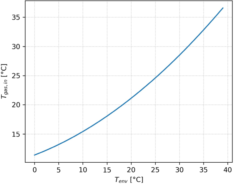
The temperature of the gas arriving at the CGS is generally unknown because of the lack of sensors at the station. Therefore, it is assumed constant in several scientific works and equal to the worst case possible [11], [12], i.e. 0 °C. In this work, a more realistic model is exploited [8], which calculates the soil temperature surrounding a pipe buried at a 1-metre depth close to the CGS according to the variation of the air ambient temperature, assuming the NG temperature inside the pipes equal to the soil temperature (18).
(17)
(18)
Figure 2 shows the NG inlet temperature increasing with the outside air temperature according to the model given by equation (17). For outside air temperature variations between 0 °C and 20 °C, the gas temperature varies between 11 °C and 21 °C. As the outside temperature decreases and drops below zero, the ground temperature stays at a minimum of around 10 °C.
Natural gas inlet temperature vs. air ambient temperature according to (17)
The temperature change the gas undergoes during an adiabatic expansion depends on the final and initial pressure states and how the expansion is carried out. In a free expansion, the gas does no work and absorbs no heat, so the internal energy is conserved. Expanding in this way, the temperature of an ideal gas would remain constant, but the temperature of a real gas decreases, except at very high temperatures. On the other hand, the Joule-Thomson expansion method is intrinsically irreversible. During this expansion, the enthalpy remains unchanged, but unlike a free expansion, work is done that causes a variation in internal energy. This change due to the irreversibility of the process means that much greater cooling or heating can be achieved than in the case of free expansion.
The Joule-Thomson effect is a phenomenon whereby the temperature of a real gas decreases following expansion conducted at constant enthalpy. In literature, this effect is often assumed constant and equal to 4−5 °C/MPa during the gas throttling process inside a CGS [11], [12], or its calculation is avoided by imposing an isenthalpic transformation between the starting point and the end point [13]. For this work purpose, the coefficient is calculated according to the following formula [19], [20]:
(19)
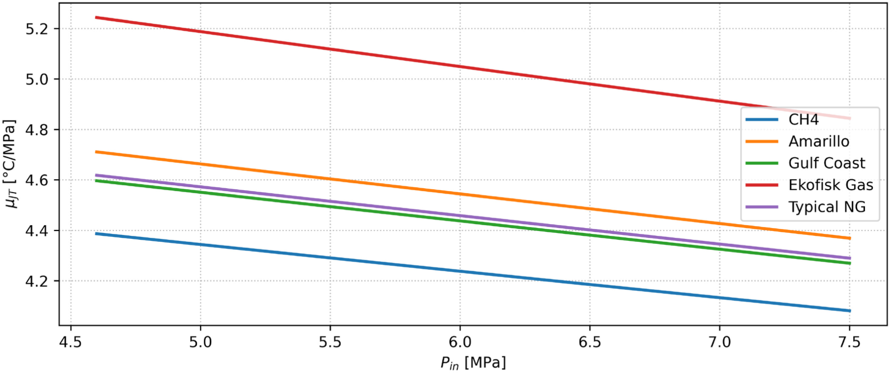
The Joule-Thomson coefficient μJT is calculated for several NG mixtures stored in the Cool Prop database [21], which are enlisted and described in Table 1. The gas outlet condition (Pout, Tout) is kept fixed and equal to the ideal set point values for pressure and several set point temperatures (30 MPa, 10 °C) to compute the isenthalpic process necessary for the μJT evaluation.
Comparison between different natural gas origins: mixture composition percentages
| Gas name | CH4 | N2 | CO2 | C2H6 | C3H8 | Iso-butane | C4H10 | Iso-pentane | C5H12 | C5H12 |
|---|---|---|---|---|---|---|---|---|---|---|
| CH4 | 100 | 0 | 0 | 0 | 0 | 0 | 0 | 0 | 0 | 0 |
| Amarillo | 90.6 | 3.12 | 0.46 | 4.53 | 0.83 | 0.103 | 0.156 | 0.032 | 0.044 | 0.039 |
| Gulf Coast | 96.5 | 0.26 | 0.60 | 1.82 | 0.46 | 0.098 | 0.101 | 0.0473 | 0.032 | 0.066 |
| Ekofisk | 85.9 | 1.01 | 1.50 | 8.50 | 2.30 | 0.349 | 0.351 | 0.051 | 0.048 | 0 |
| Typical | 95.1 | 0.09 | 2.56 | 1.84 | 0.24 | 0.040 | 0.016 | 0.014 | 0.011 | 0.08 |
Figure 3 shows the linear dependence between the Joule-Thomson coefficient, which varies approximately between 4.1 °C/MPa and 5.2 °C/MPa, and the inlet pressure for all the considered NG mixtures. Pure methane (100% CH4) is fluid with the lowest value of μ, while the Ekofisk (North European) NG is the mixture with the highest temperature drop during the throttling phase at constant enthalpy.
Joule-Thomson coefficient μJT for several gas mixtures vs. the inlet pressure Pin
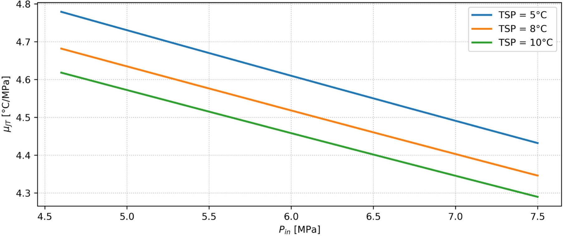
The typical NG μJT curve is chosen to be the one that will be used in the following chapters to consider a general NG mixture composition since, in Italy, there is a very high variability of gas composition due to the multitude of import origins. Focusing on the typical NG μ-curve, Figure 4 highlights the effect of a different output temperature set point on the μJT coefficient and thus on the final pre-heating energy demand. As the set point at the gas outlet increases, the temperature drops to be made by the gas at the same inlet pressure at the CGS are reduced, and thus the difference between the inlet temperature and the outlet temperature ΔTOI calculated with (11). On the other hand, a higher set point leads to an increase in the pre-heating factor calculated with (12).
Joule-Thomson coefficient μJT for the natural gas typical composition for several set points of gas outlet temperature vs. the inlet pressure Pin
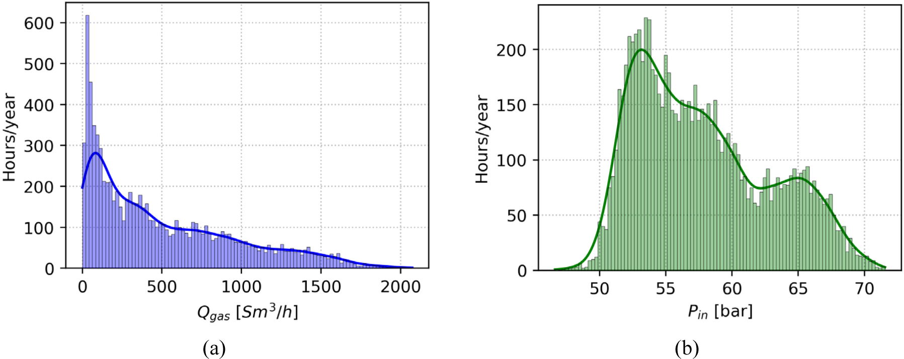
In this article, a real dataset covering one year of operation of a CGS in central Tuscany will be exploited. Figure 5a and Figure 6 show the distribution curves for the gas flow rate, the arrival pressures from the transport network, the external air temperature, and the gas outlet temperature.
Gas volumetric flow rate (a) and inlet pressure (b) examples for the considered case study
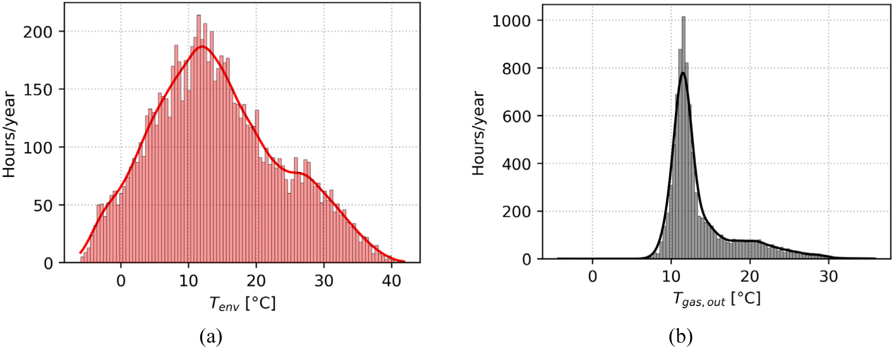
Gas temperature distribution at valve inlet (a) and valve outlet (b)
The lines of the graphs were obtained by plotting kernel density estimates to smooth the distribution and show the trend of the univariate variable. Figure 5 shows that the variation of the two input quantities, i.e., flow rate and pressure, is very wide. It is, therefore, important to consider this variation by giving the correct flow and pressure inputs to the model in equation (1).
Figure 6, on the other hand, shows the distributions of ambient temperature and, thus, of gas inlet temperature at the CGS and outlet temperature. The variation in ambient temperature is very wide and ranges from a few degrees below zero to temperatures of over 35 °C. It is interesting to assess how the gas outlet temperature follows the set point temperature set very precisely, slightly overheating compared to the set point.
The gas outlet temperature Tgas,out is the key parameter to be monitored, and it is strictly dependent on the value of the outlet temperature set point, which the DSO sets inside all the CGS. According to the Italian framework, this value must equal or exceed 5 °C. Still, for safety reasons, it is generally set at higher values and can be modulated for two working seasons: winter and summer. In this work, two different values for the outlet gas temperature are considered, replicating the actual output temperature setting inside a CGS in Italy, as can be seen in the following equation:
(20)
Figure 7 shows the layout of the CGS plant from which the annual operating data were extracted. The system includes the High Pressure (HP) inlet, two redundant lines with gas Filters (F), Preheaters (PH), gas expansion Valves (V) and the stations for Fiscal Measurement (FM) and Odorant (OD) injection before the gas is fed back into the low pressure (LP).
City gate station standard layout: red and blue lines represent hot and cold water, dark blue lines natural gas
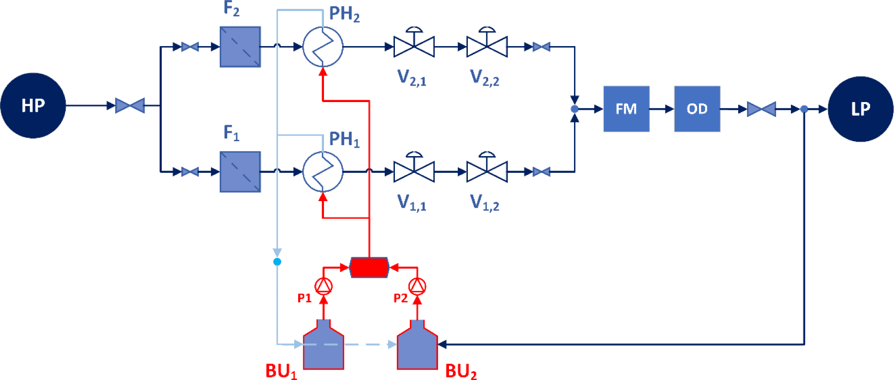
The control logic of the installed system does not provide for an inverter-controlled flow rate, as assumed in the theoretical study, but a constant value of the pre-heating water flow rate regardless of the gas conditions at the CGS inlet. It affects pre-heating efficiency, as the minimum flow rate of water required for pre-heating is never supplied, and the two pumps (P1 and P2) always run at constant revolutions and process the same water flow rate. The boilers operate alternately: the one that does not operate remains on stand-by and consumes an almost constant amount of gas for the pilot flames of approximately 0.25 Sm3/h.
The model used to calculate pre-heating gas consumption was refined by adding improving assumptions. The hypotheses that have been gradually added are as follows:
Hp1: Variable gas flow rate crossing the CGS instead of a single constant value,
Hp2: Real outlet temperature set point according to DSO,
Hp3: Variable gas inlet pressure,
Hp4: Variable gas inlet temperature depending on ambient air temperature with the model of equation (9).
Another important hypothesis concerns the control logic of the pre-heating system: to generalise the work as much as possible and after talking with the DSO, it was decided to follow a logic based on modulation of the water flow rate according to the heat supplied to the gas.
Once the water flow temperature to the PH is fixed and the gas conditions are known, the flow rate is derived accordingly to match the thermal demand at PH perfectly.
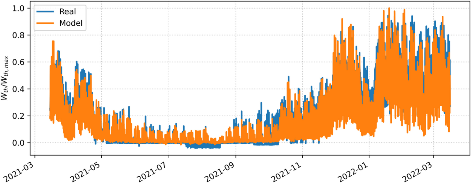
Figure 8 and Figure 9 present the results of comparing the hourly trends of the thermal load output calculated with the model throughout the year and during four typical days, respectively. The demand curves of the model and the real data are dimensionally adjusted for confidentiality reasons and to make the treatment generic for any CGS: the model with real inputs can faithfully replicate consumption trends for all seasons of the year, as seen in the abovementioned figures.
Hourly required dimensionless thermal power: model vs. real data during one year
Daily comparison between the hourly required dimensionless thermal power: final model vs. real data for four different seasons
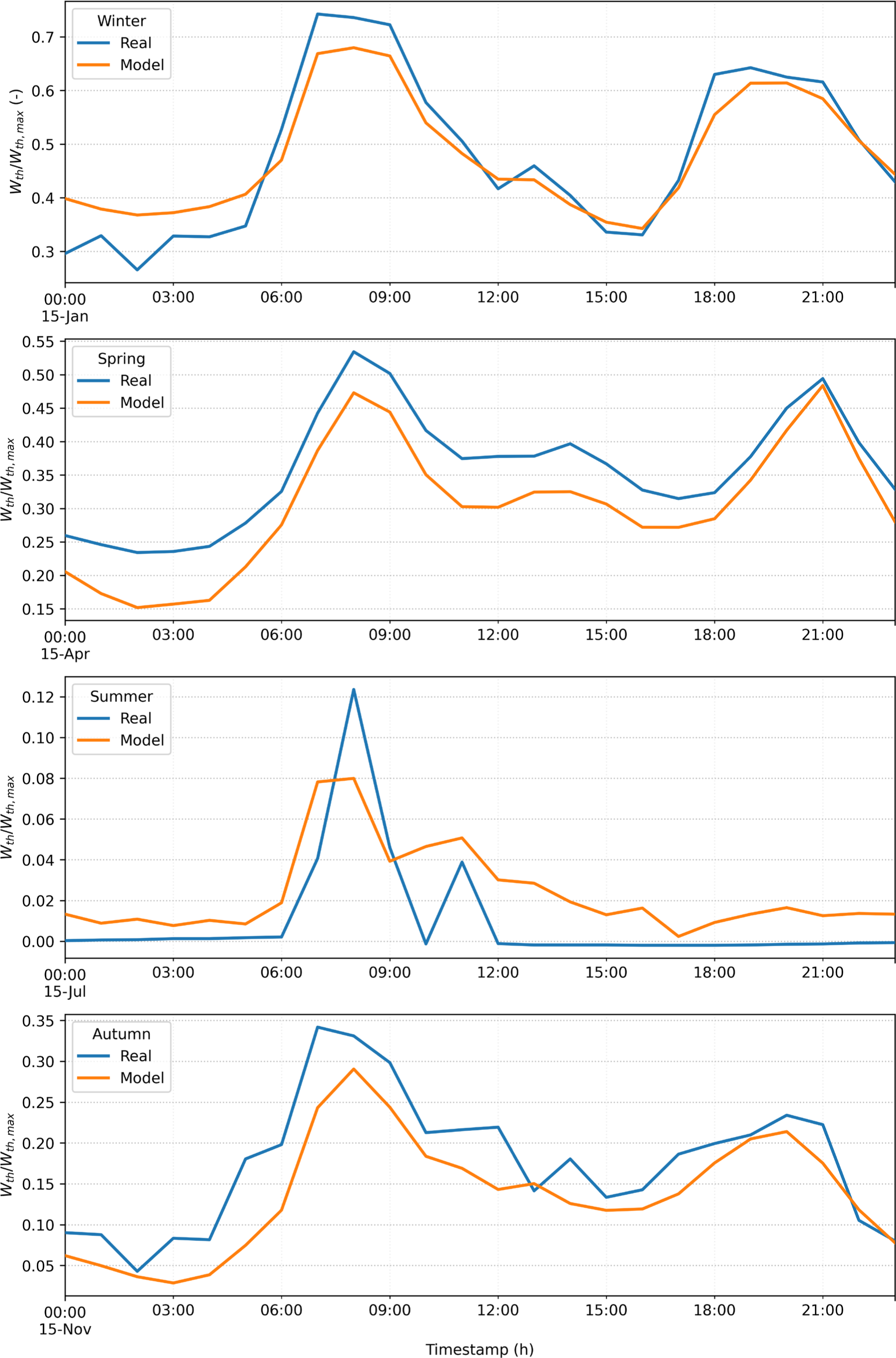
Figure 9 shows that the model is very accurate during system operation at maximum load (peak daytime hours and winter seasons). On the other hand, the model tends to under- or over-estimate at other times of the day, particularly at night and in summer, when the gas flow rate is very low, and the plant presumably retains a certain amount of heat loss. It can be seen from the figures that the operation of the cabin is highly influenced by the OCs in which it operates: when it is at maximum load, the relationship in equation (1) between consumption Wgas and gas flow rate Qgas, with all the assumptions added during the development of the model, is optimal.
In the intermediate seasons (autumn and spring), there is a slight underestimation of the typical days shown in Figure 9. For summer, when the gas inlet temperature is very high, the model still estimates a certain theoretical percentage of gas to be burned when it is possible that in real OCs, the cabin exploits thermal inertia to avoid turning on the boilers at times of lower demand. The demand curve used in the following paragraphs is obtained by multiplying the validated dimensionless curve of Figure 8 by the peak power value of 28,738 kW.
Table 2 enlists each improving hypothesis assumed to compute the annual thermal energy consumption with the proposed model. Including a realistic, not estimated, constant flow rate throughout the year, the performance of the thermodynamic model increases significantly (from 413 MWh to about 101 MWh). The following hypotheses allow us to reduce the forecasting from 101 MWh to 74 MWh (Hp2), then to 53 MWh (Hp3) and finally to reach a value of Egas,y of about 44 MWh.
Pre-heating consumption models’ hypotheses
| Model ID | Qgas | Tgas,out | Pgas,in | Tgas,in |
|---|---|---|---|---|
| BL (Base Load) | Design (max) | Max (10 °C) | Max (7.5 MPa) | Min (0 °C) |
| BL + Hp1 | Real Qt | Max (10 °C) | Max (7.5 MPa) | Min (0 °C) |
| BL + Hp1 , Hp2 | Real Qt | Real Set Point (10 & 8 °C) | Max (7.5 MPa) | Min (0 °C) |
| BL + Hp1 , Hp2 , Hp3 | Real Qt | Real Set Point (10 & 8 °C) | Real Pin(t) | Min (0 °C) |
| Final Model | Real Qt | Real Set Point (10 & 8 °C) | Real Pin(t) | Tgas,in=f(Tenv) |
The PV field simple model is taken from the Energy Plus 8.0 database, and thus the every-hour electrical power is given by the following equation:
(21)
Where G(t) is the total solar incident irradiation on the solar panel [W/m2], APV is the solar panels’ total area [m2], ηPV and ηloss are the efficiencies of the panels and the inverter system, respectively, and fcell is the fraction of usable cells. For this work, the three latter parameters are assumed constant and equal to 0.2, 0.98, and 0.95.
The HP is a very efficient technology for heating and cooling purposes since its efficiency, expressed by the COP (Coefficient of Performance), usually varies from 2 to 5 and is particularly high when used to heat a utility or process. The value of the COP is calculated according to (22), considering the efficiency dependence on the temperature difference between the water supply temperature and the ambient air temperature ΔTHP [22].
(22)
(23)
The real COP is then obtained by a correction on the previous formula, which is given for reference value of COPref equal to 3.9, including the value of the ideal COP of the considered HP model COPdes.
(24)
The case study analysis results presented in the previous chapters are described below. First, the results of the technical analysis are presented in terms of energy savings evaluations. Next, the results of the economic analysis are presented.
Figure 10a describes the percentage of annual thermal energy saved as a function of photovoltaic panel size. The analysis is conducted by installing different sizes of photovoltaic panels ranging from a minimum of 10 m2 to a maximum of 150 m2. Assuming a total efficiency given by the product of the efficiencies used in equation (21), this area span will correspond to an installed kWp value that will then be used to calculate the economic investment. The installed kWp will vary between about 2 and about 30. In any case, the theoretical maximum value of the percentage of energy that can be saved has been identified as 53 % of the total thermal energy.
Percentage of annual energy saved compared to total energy required from gas (a) and SSR and SCR variation (b), according to photovoltaic size
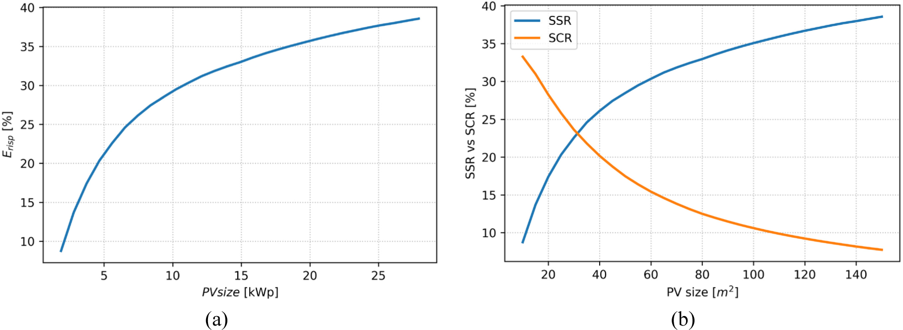
Jedilkowski et al. [12]conducted a study very similar to the one proposed, and the maximum percentage of recoverable energy from their system (air source heat pump) is 53%, compared to their proposal, which is higher at around 60-70%. Englart et al. [11] propose a similar assessment with ground source heat pumps; in this case, the maximum amount of recoverable energy comes to 44% of the total energy required for pre-heating and is lower than the maximum amount recoverable by the system proposed in this article.
The trends of the SSR and SCR parameters are shown in Figure 10b. The value of the SSR perfectly follows the trend of the percentage of energy saved in Figure 11a. The SCR coefficient highlights that after a certain size of the installed panel, approximately 30 m2, the energy not used to reduce the thermal load of the pre-heating exceeds that used by the heat pump. It results from the photovoltaic production curve peaking when the gas demand curve has its minimum. Consequently, increasing the size of the photovoltaic system with this layout only leads to a small gain in thermal energy saved and a large increase in energy produced by the panel that must be curtailed or possibly sold to the grid.
The total volume of gas annually saved when varying the size of the photovoltaic system (a) and relative number of energy efficiency certificates gained (b)
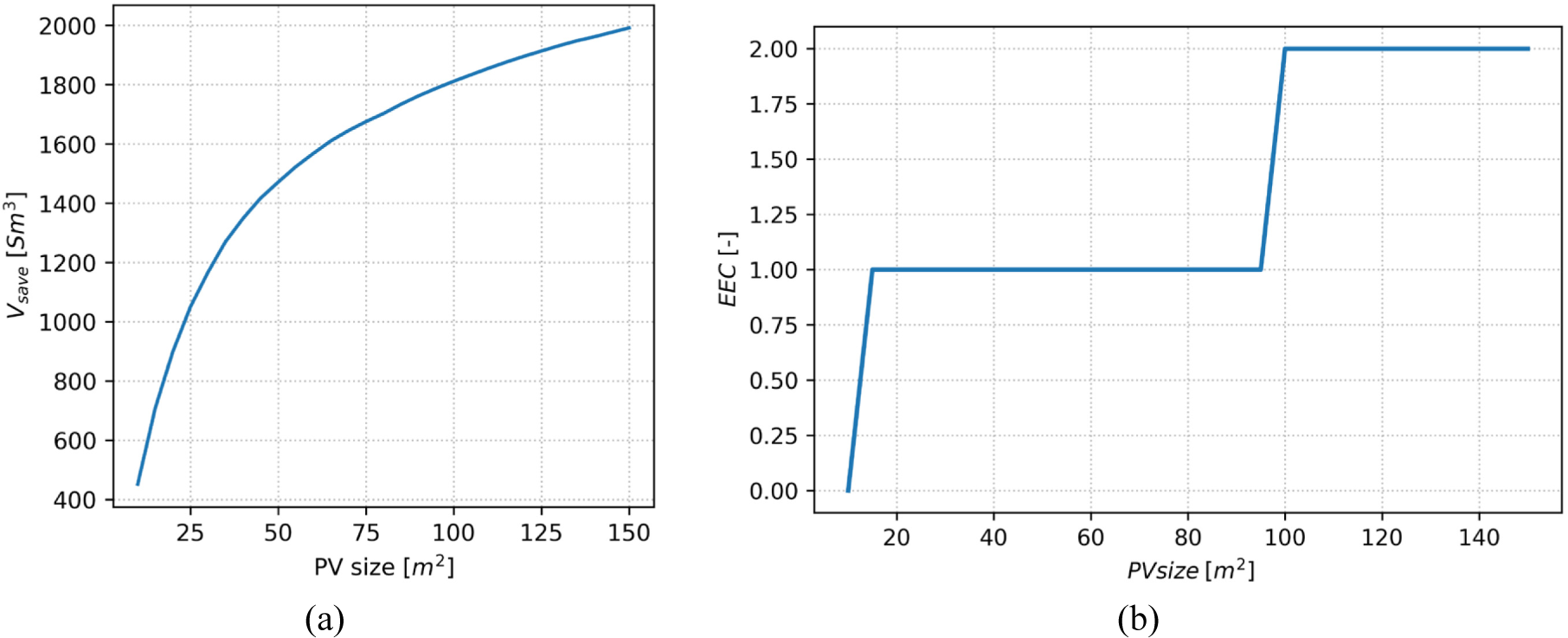
The first step in the economic evaluation is to calculate the number of Energy Efficiency Certificates (EECs) one can access based on the volume of natural gas saved in the year, expressed in tonnes of oil equivalent (TOE) [23].
A certificate is awarded for each TOE of natural gas, using the conversion between Sm3 of NG and TOE and approximating this value by default if the TOE unit is less than half or by excess if equal or greater. For this work, a conversion factor of 0.836 TOE per 1000 Sm3 of natural gas saved was chosen. Figure 11 shows the volume of gas in standard cubic metres that can be saved for each installed PV panel size and heat pump size accordingly, and the number of certificates accessed. Between 10 m2 and 12 m2, one gets no certificate; between 13 m2 and 96 m2, one gets 1 certificate; between 97 m2 and 150 m2, one gets 2 certificates.
Table 3 shows all the assumptions chosen for the economic feasibility assessment. Regarding photovoltaic installation prices, reference is made to an average of various prices found in the literature, for example, [24], [25]. The total operating cost of the PV is obtained from [26] and set equal to 1% of the total investment. The replacement time of the inverter is set at 15 years, as generally proposed in the literature. For the HP cost, given the enormous variability of the available prices, a value of 400 €/kWth was chosen as a reference, as suggested by [27] under the assumption of using a reasonable value assumed for heat pumps for decarbonisation of industrial processes, such as this case. Regarding electricity sales prices, they were based on a typical minimum guaranteed price provided by the national regulators [23]. With the assumptions in Table 3, the initial investment and annual cash flows are calculated using equations (25) and (26), where WPV,peak and WHP,peak stand for the PV field and HP peak size chosen for each case.
Values selected for the economic assessment
| Component/Tariff | Symbol | Unit | Value |
|---|---|---|---|
| PV overall installation costs | CPV | [€/kWp] | 1500 |
| HP installation cost | CHP | [€/kWth] | 400 |
| HP O&M | CHP, O | [%] | 1.5 |
| PV O&M | CPV,O | [%] | 1 |
| PV inverter lifetime | ninv | [year] | 15 |
| EEC value | CEEC | [€/unit] | 250 |
| EEC years | nEEC | [year] | 7 |
| Gas sales price | CNG | [€/Sm3] | 1 |
| Electricity sales price | Cel | [€/kWh] | 0.05 |
| Discount rate | i | [%] | 6 |
(25)
(26)
The NPV is finally calculated using the following formula:
(27)
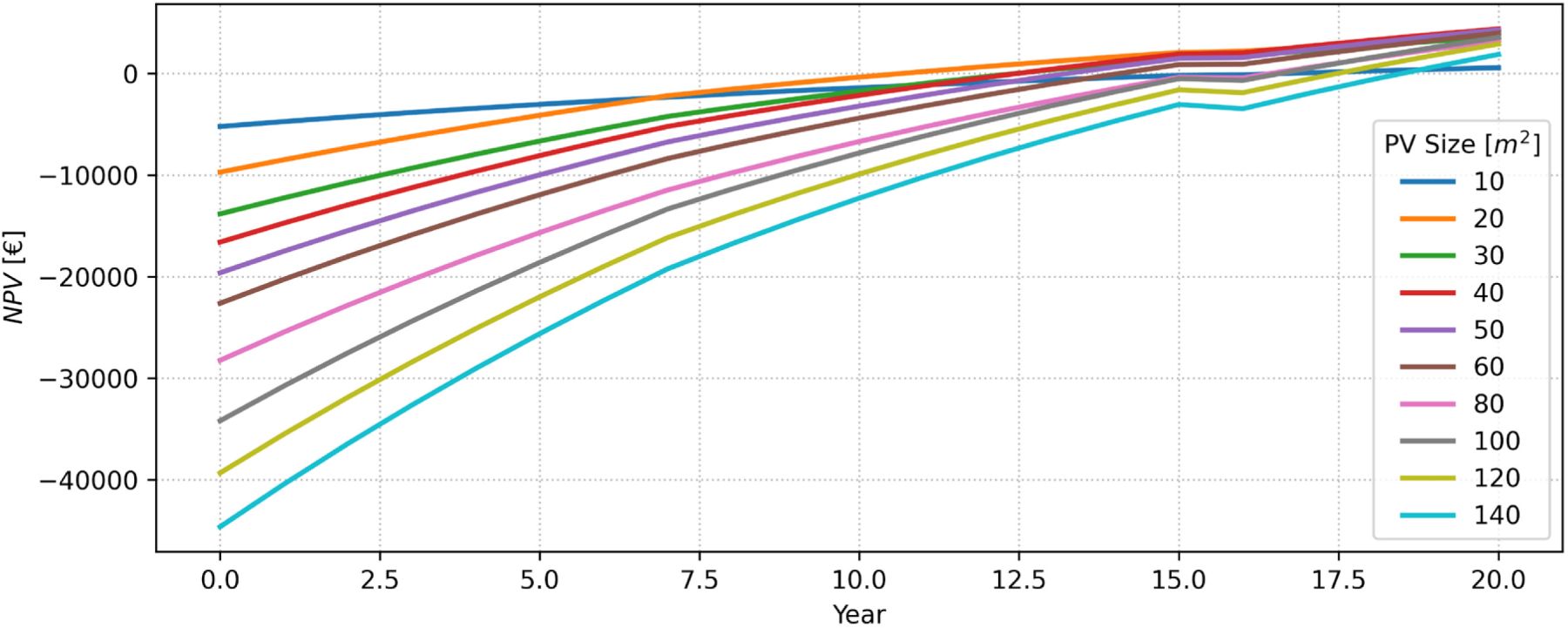
When the period of the certificates expires, they are removed from the annual cash flow. Figure 12 presents the NPV values for the entire investment lifetime n (20 years) as the size of the solar system varies. The EEC parameters affect the payback time of the investment, especially in the case of sizes larger than 100 m2 since it is possible to access up to twice as many certificates, which is why the first seven years present a steeper curve than the cases of sizes smaller than 100 m2. With a size range from 10 m2 to 13 m2, one is not eligible for certificates, so the investment is not very profitable. A certificate is granted for values above 13 m2, and the curves gain profitability. From the 15th year, the effect of inverter replacement is visible, penalising the investment as the size increases.
present value over the life of the investment for various sizes of installed photovoltaics
The simple payback time (PBT) is calculated as the first year where the NPV is higher than zero.
(28)
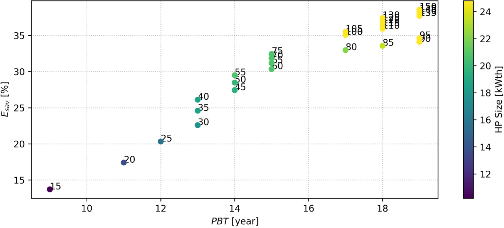
Figure 13 shows the values of the total percentage energy saved in the year and the PBT of the investment as a function of photovoltaic size (dots annotations) and heat pump size (dots colours ranging from dark to light). The chart only considers cases accessing at least one EEC. The recoverable thermal energy increases with the investment, and thus, with the simple PBT payback time, within the PBT ranges, there are various configurations of photovoltaic panel and heat pump sizes. Consequently, different amounts of energy can be recovered with the same PBT. Between 30 and 40 m2, there is an inversion of the NPV curve trend: the higher investment is justified by a cash flow that allows the investment to be recovered in about the same time and a slightly higher NPV in the last year. There is also a clear reduction in PBT from 95 to 100 m2, the threshold for access to the second EEC. The jump between 15 and 17 years of PBT is because of inverter replacement, which occurs between years 15 and 16.
Simplified payback time for various sizes of installed PV
From an economic point of view, the results presented above can be compared with works applying different technologies to plants of a similar size. Volumetric expanders [13] make it possible to recover about 15% of the energy and up to a maximum of 25/27% with a PBT of about 4 years. The application of Ranque–Hilsch vortex technology [14] is more difficult to evaluate because the working temperature influences it; still, it is generally possible to recover up to 33% of the energy with a PBT of less than 10 years.
The proposed system, consisting of a combination of auxiliary boiler and heat pump powered by a photovoltaic field, has the following advantages and disadvantages:
Advantages: simple system, easily controllable, decarbonisation is achieved through high-efficiency technologies (heat pumps have a thermal efficiency ranging between 2.5 and 4) and allows access to EECs for DSO.
Energy sustainability: compared to conventional systems, the proposed one could save up to 3 tonnes of CO2 equivalent from unburned natural gas per year.
Disadvantages: the curves of electricity production from photovoltaic panels and demand for pre-heating gas are strongly decoupled, which leads to a maximum decarbonisation limit of the process with the proposed layout.
A viable improvement would be to add a seasonal storage system, relying, for example, on a hydrogen production and storage system, which could be converted back into energy via a hydrogen boiler or fuel cell. In addition, this configuration would also allow a surplus of green gas to be injected directly into the network and immediately downstream of the CGS, an ideal point for injecting this type of gas because it would not require the energy cost of recompression and because it would limit the effect of gas quality variation on end-users.
Through a techno-economic analysis, this article clarifies the feasibility of decarbonising the natural gas pre-heating process in CGS using a heat pump powered by renewable sources.
The main outcomes of the work are:
The development of a simplified thermodynamic model improved and calibrated with real data, allows a sufficiently accurate estimate of the ideal annual thermal energy needed for gas pre-heating inside a CGS, considering all effects due to actual operating conditions. The method can be used for each CGS, providing the input data specified in the work.
The amount of thermal energy that can be recovered through these hybrid systems without overcoming the excessive energy waste is around 22% of the total annual thermal energy according to SSR and SCR parameters. The maximum recoverable percentage, in any case, could be around 53% of the total annual energy required due to the mismatch between the demand and production curves of photovoltaics.
Increasing the size of the photovoltaic system pays off only up to a certain maximum, identified as around 40 m2, for which the NPV at 20 years is the maximum. After this value, the investment’s payback time increases, the NPV at 20 years decreases, and the effect of energy efficiency certificates is less than for smaller sizes.
For the considered size range of the photovoltaic system, up to 38% of the energy can be recovered with a PBT of less than 20 years, up to 32 % with a PBT of less than 15 years and up to 26% with a PBT of about 13 years.
Future developments of this work will be applying this general method to more classes of CGS for an overall evaluation on a regional or national scale.
The authors acknowledge Centria S.r.l. for the support and the data supply.
- ,
Assessing the total theoretical, and financially viable, resource of biomethane for injection to a natural gas network in a region ,Applied Energy , Vol. 188 ,pp 237–256 , 2017, https://doi.org/https://doi.org/10.1016/j.apenergy.2016.11.121, February - ,
Steady-state analysis of a natural gas distribution network with hydrogen injection to absorb excess renewable electricity ,International Journal of Hydrogen Energy , Vol. 46 (50),pp 25562–25577 , 2021, https://doi.org/https://doi.org/10.1016/j.ijhydene.2021.05.100, July - ,
Hydrogen blending in the Italian scenario: Effects on a real distribution network considering natural gas origin ,Journal of Cleaner Production , Vol. 379 ,pp 134682 , 2022, https://doi.org/https://doi.org/10.1016/j.jclepro.2022.134682, December - ,
Environmental baseline monitoring for shale gas development in the UK: Identification and geochemical characterisation of local source emissions of methane to atmosphere ,Science of The Total Environment , Vol. 708 ,pp 134600 , 2020, https://doi.org/https://doi.org/10.1016/j.scitotenv.2019.134600, March - ,
Thermal modeling of indirect water heater in city gate station of natural gas to evaluate efficiency and fuel consumption ,Energy , Vol. 212 ,pp 118390 , 2020, https://doi.org/https://doi.org/10.1016/j.energy.2020.118390, December - ,
Data-driven modelling for gas consumption prediction at City Gate Stations ,J. Phys.: Conf. Ser. , Vol. 2385 (1),pp 012099 , 2022, https://doi.org/https://doi.org/10.1088/1742-6596/2385/1/012099, December - ,
Feasibility of accompanying uncontrolled linear heater with solar system in natural gas pressure drop stations ,Energy , Vol. 41 (1),pp 420–428 , 2012, https://doi.org/https://doi.org/10.1016/j.energy.2012.02.058, May - ,
Integration of vertical ground-coupled heat pump into a conventional natural gas pressure drop station: Energy, economic and CO2 emission assessment ,Energy , Vol. 112 ,pp 998–1014 , 2016, https://doi.org/https://doi.org/10.1016/j.energy.2016.06.100, October - ,
Energy recovery from natural gas pressure reduction stations: Integration with low temperature heat sources ,Energy Conversion and Management , Vol. 159 ,pp 274–283 , 2018, https://doi.org/https://doi.org/10.1016/j.enconman.2017.12.084, March - ,
Key performance indicators for integrated natural gas pressure reduction stations with energy recovery ,Energy Conversion and Management , Vol. 164 ,pp 219–229 , 2018, https://doi.org/https://doi.org/10.1016/j.enconman.2018.02.089, May - ,
Renewable energy sources for gas pre-heating ,E3S Web Conf. , Vol. 116 ,pp 00019 , 2019, https://doi.org/https://doi.org/10.1051/e3sconf/201911600019 - ,
Reducing energy consumption for electrical gas pre-heating processes ,Thermal Science and Engineering Progress , Vol. 19 ,pp 100600 , 2020, https://doi.org/https://doi.org/10.1016/j.tsep.2020.100600, October - ,
Thermodynamic and Economic Feasibility of Energy Recovery from Pressure Reduction Stations in Natural Gas Distribution Networks ,Energies , Vol. 13 (17),pp 4453 , 2020, https://doi.org/https://doi.org/10.3390/en13174453, August - ,
A Smart Energy Recovery System to Avoid Pre-heating in Gas Grid Pressure Reduction Stations ,Energies , Vol. 15 (1),pp 371 , 2022, https://doi.org/https://doi.org/10.3390/en15010371, January - ,
Multi-objective optimisation of pre-heating system of natural gas pressure reduction station with turbo-expander through the application of waste heat recovery system ,Thermal Science and Engineering Progress , Vol. 38 ,pp 101509 , 2023, https://doi.org/https://doi.org/10.1016/j.tsep.2022.101509, February - ,
An experimental investigation on using heat pipe heat exchanger to improve energy performance in gas city gate station ,Energy , Vol. 252 ,pp 123959 , 2022, https://doi.org/https://doi.org/10.1016/j.energy.2022.123959, August - ,
Quantifying self-consumption linked to solar home battery systems: Statistical analysis and economic assessment ,Applied Energy , Vol. 182 ,pp 58–67 , 2016, https://doi.org/https://doi.org/10.1016/j.apenergy.2016.08.077, November - ,
Snam home page” , , https://www.snam.it/it/index.html, [Accessed: 12.03.2023] - ,
Influences of Hydrogen Blending on the Joule–Thomson Coefficient of Natural Gas ,ACS Omega , Vol. 6 (26),pp 16722–16735 , 2021, https://doi.org/https://doi.org/10.1021/acsomega.1c00248, July - ,
Effects of natural gas compositions on its Joule–Thomson coefficients and Joule–Thomson inversion curves ,Cryogenics , Vol. 111 ,pp 103169 , 2020, https://doi.org/https://doi.org/10.1016/j.cryogenics.2020.103169, October - ,
Pure and Pseudo-pure Fluid Thermophysical Property Evaluation and the Open-Source Thermophysical Property Library CoolProp ,Ind. Eng. Chem. Res. , Vol. 53 (6),pp 2498–2508 , 2014, https://doi.org/https://doi.org/10.1021/ie4033999, February - ,
A review of domestic heat pumps ,Energy Environ. Sci. , Vol. 5 (11),pp 9291–9306 , 2012, https://doi.org/https://doi.org/10.1039/C2EE22653G, October - ,
ARERA - Home page” , , https://www.arera.it/it/index.htm, [Accessed: 12.03.2023] - ,
Decarbonising heat with PV-coupled heat pumps supported by electricity and heat storage: Impacts and trade-offs for prosumers and the grid ,Energy Conversion and Management , Vol. 240 ,pp 114220 , 2021, https://doi.org/https://doi.org/10.1016/j.enconman.2021.114220, July - ,
Impact of PV and variable prices on optimal system sizing for heat pumps and thermal storage ,Energy and Buildings , Vol. 128 ,pp 723–733 , 2016, https://doi.org/https://doi.org/10.1016/j.enbuild.2016.07.008, September - ,
A European Assessment of the Solar Energy Cost: Key Factors and Optimal Technology ,Sustainability , Vol. 13 (6),pp 3238 , 2021, https://doi.org/https://doi.org/10.3390/su13063238, March - ,
The future of low carbon industrial process heat: A comparison between solar thermal and heat pumps ,Solar Energy , Vol. 173 ,pp 893–904 , 2018, https://doi.org/https://doi.org/10.1016/j.solener.2018.08.011, October