Solar photovoltaic (PV) modules are designed to attract the solar irradiance and transfer it to electrical power. The performance of PV depends on the amount of the solar irradiance hitting the modules [1]. The solar companies test the modules at standard test conditions (STC) of 1000 W/m2 solar irradiance, 25 °C cell temperature, and 1.5 air mass [2]. During this test, the focus is to identify the output electrical characteristics of the PV modules. These are the open circuit voltage (Voc), short circuit current (Isc), maximum power point voltage (Vmp) and current (Imp), fill factor (FF), maximum power (Pmax) and efficiency. Undoubtedly, there is a number of environmental and operational factors that would prevent the PV modules from capturing the maximum solar irradiance or operating at their nominal efficiencies [3]. Specifically, the variations of solar irradiance [4], thermal effect due to ambient temperature [5], soiling effects [6], partial shading, wind speed [7], humidity ratio [8] and module degradation [9] are all considered as essential influencers. For instance, the high solar irradiance has a prominent impact on the output power of PV module. However, the low solar irradiance causes a nonlinear reduction in the short circuit current and then reduces the module output power [10]. Accordingly, the performance of PV modules differs significantly under variable light conditions, depending on the geographic position of the PV installation, changing atmospheric conditions [11] and changing position of the sun (solar inclination) [12]. Furthermore, the open circuit voltage of a PV module depends strongly on the module temperature and overheating causes a decrease in the produced energy [13]. Whereas, the accumulation of soiling on the module surface impacts PV performance by inhomogeneous or homogenous shading [14] especially during the period of dry climate [15]. Besides, non-uniform distribution of soils on the surface of PV modules causes shading of cells resulting in an increase in the modules temperature and then leading to create hot spots [16]. In this regard, it should be noted that the PV modules are spectrally selective and therefore, their performance is influenced by the changes in the solar spectrum distribution caused by scattering and absorption in the atmosphere [17]. In a summary, there is a consistent and tangled relationship between the operational conditions and the generated power of PV module. An increase in solar radiation would increase the power. However, an increase in module temperature causes an increase in the current with a sharp decrease of voltage and a drop of power [18]. This action can be mitigated with a higher wind which would cool the PV’s surface and enhance its performance [19] or by combination between PV module and thermal solar collector that called photovoltaic-thermal collector (PV/T) [20]. Accordingly, a number of scientists attempted with triggered motivation to conduct modeling of PV modules considering the interactions between the inlet conditions and performance metrics.
In last decade, the implementation of PV forecasting methods has become an active research field to predict the generated power of PV. Numerous techniques were utilised to predict and optimise the generated power of PV modules under the various operation conditions while considering different types of PV modules and the available data. These techniques can be classified into a) a physical technique (model based method) and b) a statistical technique (model based historical data) [21]. In the model based method, the numerical weather prediction model is used to predict the weather variables including the solar irradiance, ambient temperature and wind speed, which are corroborated to estimate the generated power of PV module [22]. On the other hand, the statistical techniques, such as Linear Regression (LR) model [23], a multiple linear regression (MLR) [24], autoregressive (AR) model [25], Moving Average (MA) model [26] Machine Learning (ML) models like Artificial Neural Network (ANN) [27], and Response Surface Methodology (RSM) [28], are developed based on measured data over a period of time. Generally, the numerical weather prediction models are more suitable for a long predict horizons, while the statistical models are indicated for short horizons. Moreover, the statistical model can overcome all the difficulties in physical model. Therefore, the statistical model is simpler than physical model. Specifically, the fitting equations developed based on available empirical data require less input data and less computation efforts for the prediction of power generated. Among all statistical techniques, LR is a relatively simple technique that may be carried out quickly and reliably as compared to some of the other ML methods due to ability in much reducing time complexity. The RSM was utilised by several colleagues to model and optimise the performance indicators of various industrial processes [29]. For instance, the results of an experimental examination into the impacts of cutting speed, feed rate, depth of cut, nose radius, and cutting environment in CNC turning of AISI P-20 tool steel were published by Aggarwal et al. [30]. The goal of the experimental investigation has been achieved using the RSM and Taguchi's approach. Furthermore, an accurate model was created by Al-Obaidi et al. [31] to forecast the dimethylphenol removal from wastewater using the reverse osmosis technique. Based on real experimental data gathered from the literature, the RSM was specially used to carry out this challenge. In this regard, a precise investigation to explore the efficiency of RSM based mathematical model to precisely predict the power generated of photovoltaic panel considering the influence of essential control variables has not yet been established and hence demonstrates the novelty of this study. Accordingly, the main aim of this study is to deploy the RSM based on the D-optimal Design (DOD) approach to model an optimise the generated power of PV module using desirability function. The interaction of three essential independent parameters including: solar irradiance 169.2 - 981.7 W/m2, module temperature 36.14 - 67.01 °C and wind speed 0.5 - 2.4 m/s with the dependent variable, is considered through the process modelling and optimisation. The suggested response model used two factorial (2FI) order with polynomial equation.
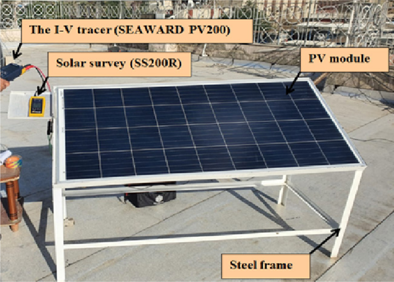
In this study, a polycrystalline PV module type (Protonix Fotuner India FRS-165 W) was selected to test and collect the data. The PV module was installed on the rooftop of Mechanical Engineering Department at Baqubah Technical Institute-Middle Technical University (latitude of 33.7733° N and longitude 45.1495° E). The tested module is shown in Figure 1. The technical specifications of PV module are summarized as: (Pmax=165 W, Isc=9.81 A, Voc=22.05 V, Imp=9.17 A, Vmp=18 V, efficiency η=20% and temperature coefficient of maximum power=-0.45%/°C). The module was mounted on steel structure inclined at 33° as a tilt angle. The module was monitored by I-V tracer (SEAWARD PV200), solar survey (SS200R) and wind speed meter (anemometer) throughout August of 2023.
Tested PV module of nominal power 165 W
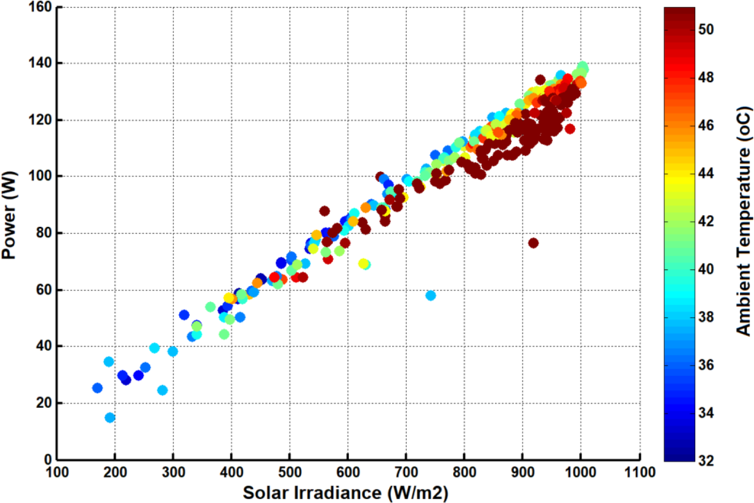
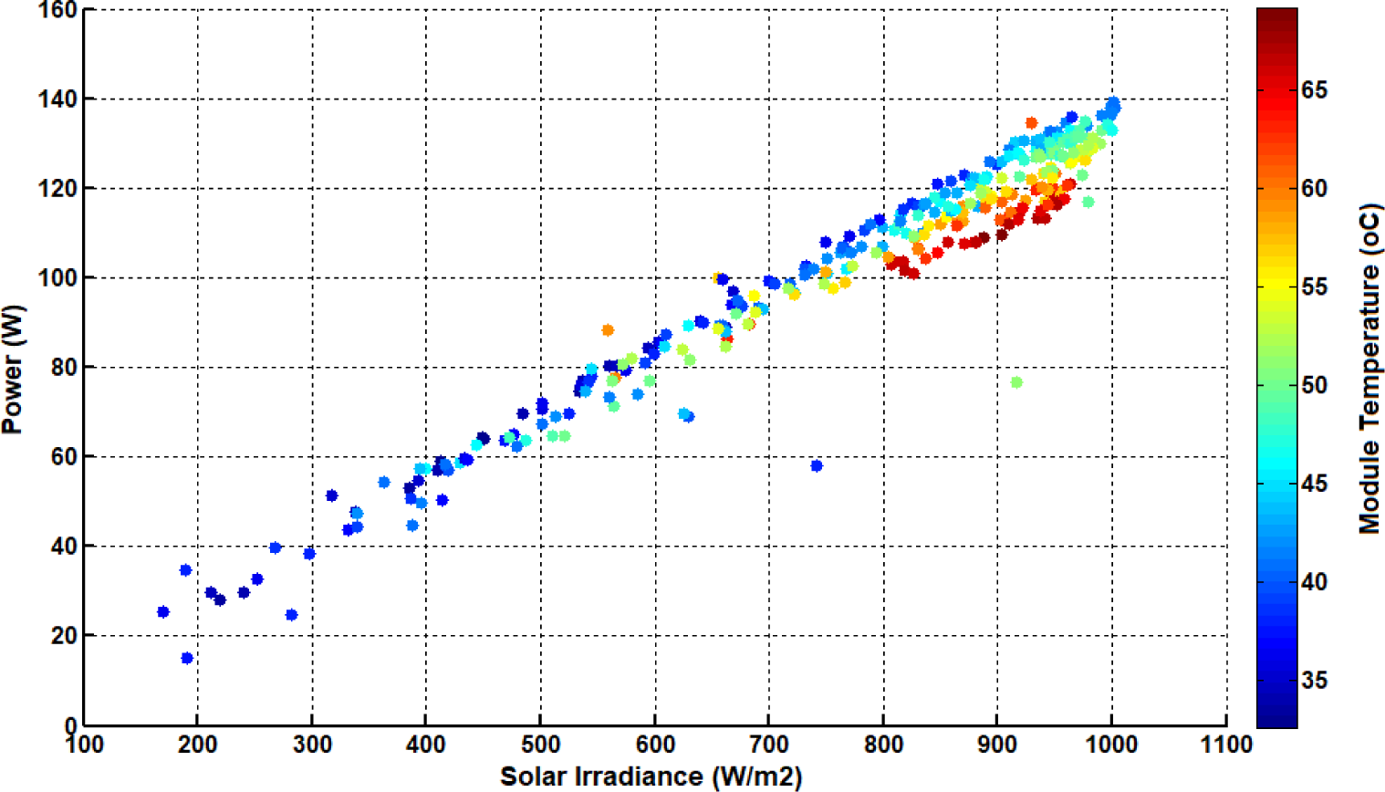
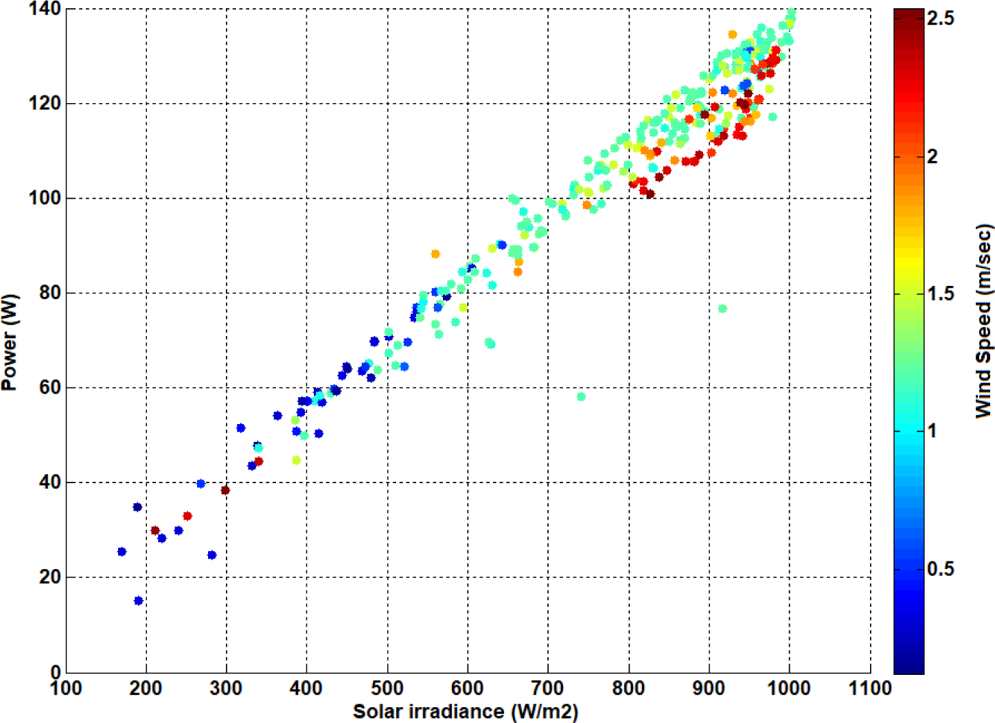
In order to verify the proposed RSM model, an outdoor experiment was performed to collect number of datasets. These datasets were collected every five minute including: the solar irradiance, ambient temperature, wind speed and module temperature. In addition, the output electrical characteristics of PV module (ISC, VOC, Imp and Vmp) were measured to calculate the output power. The collected data are plotted as depicted in Figures 2, 3 and 4. Specifically, the output power of PV module is plotted against the solar irradiance under the influence of both ambient and module temperature and wind speed. The representation of these data are convenient to illustrate the wind speed effect in cooling of PV module and then enhances its power [32]. The PV power has witnessed a progressive as a result to increasing solar irradiance. This increase is significant when the module temperature is low due to an increase in wind speed.
DC power of PV module against solar irradiance and ambient temperature measured by the experimental tests
DC power of PV module against solar irradiance and module temperature measured by experimental tests
DC power of PV module against solar irradiance and wind speed measured by experimental tests
A statistical technique is called Response Surface Methodology (RSM). It is utilised for creating models, designing tests, and examining the connections between various factors. RSM is frequently used to optimise processes, enhance product quality, and comprehend complicated systems in a variety of disciplines, including engineering, chemistry, and biology. To depict the link between input variables (factors) and output responses, statistical models are created in RSM. By identifying the ideal mix of input variables, these models can be utilised to optimise the responses and forecast how a system would behave within the experimental zone. To fit mathematical models to the observed responses, examine experimental data, and derive conclusions regarding the relationships between variables, RSM uses statistical techniques [33].
In this study, the D-Optimal Design (DOD) approach was employed with solar irradiance, module temperature and wind speed as independent variables. In this regard, the generated power of PV module was the response variable. Mathematically, the relationship between the response and the independent variables can be represented as [34]:
(1)
Y and X are the response and the independent variables. k is the number of independent variables and ε is the error of them.
Two factorial (2FI) response model with the polynomial equation were used to explain the relationship between the dependient and independent variables based on the multiple linear regression analysis taking into account the main and the interaction impact of independents on the genearted power. The values of the independent variables are transformed into code variables and represented as: [-1, 0, +1] depending on its relative distance from the central value point. Table 1 shows the summary of the transformation of the actual variables into code variables. This model take in cosideration the sequential sum of squares for the two-factor interaction (X1X2, X2X3 and X1X3) terms. The F-value tests the significance of adding interaction terms to the linear model [35]. A small P-value (Prob>F) indicates that adding interaction terms has improved the model. According to the above proposed model, the value of generated power is represented in the counter of eq. (2) [36]:
(2)
Codes and variables values in two factorial order model
| Parameters | Code | Symbol | Unit | Code in 2F1 design | ||
| -1 | 0 | 1 | ||||
| Solar Irradiance | X1 | S | W/m2 | 169.2 | 575.45 | 981.7 |
| Module Temperature | X2 | Tpv | °C | 36.14 | 51.58 | 67.01 |
| Wind Speed | X3 | V | m/s | 0.5 | 1.45 | 2.4 |
To evaluate the accuracy of the proposed model, some of the statistical indicators were used through a comparison between the predict and actual values. The most important indicators under consideration are the Mean Square Error (MSE), coefficient of determination (R2) and absolute relative error [37]. The MSE value is calculated by [38]:
(3)
i is the number of variables, N is the number of data points, Yi and are the actual and predicted values, respectively.
R2 can be calculated using eq. (4) [39]:
(4)
RSS and TSS are the residual and total sum of squares and can be defined as [39]:
(5)
(6)
is the mean value of a sample. The absolute relative deviation (ARD) is calculated by [40]:
(7)
Based on the experimental data that obtained through testing the PV module, three relevant parameters were used in the experiments to predict and optimise the generated power of PV module using RSM. The D-optimal design (DOD) technique was used for analyzing the case study. The solar irradiance, module temperature and wind speed have been considered the three relevant parameters each one has three levels.
The results of model regression are analyzed and evaluated in Table 2. The summary fit of Sequential Model Sum of Squares and model statics are performed for the selected model of power generated of PV module. It can be observed that a Quadratic and 2FI model was chosen based on the probability value (P-value) of the various models under consideration (<0.0001).
Fit summary of the two factorial order model
| Sequential model sum of squares | ||||||
|---|---|---|---|---|---|---|
| Source | Sum of squares | df | Mean square | F-value | P-value | Remark |
| Mean | 2.156*10+5 | 1 | 2.156*10+5 | |||
| Linear | 26582.34 | 3 | 8880.78 | 466.66 | <0.0001 | |
| 2FI | 246.48 | 3 | 82.16 | 7.92 | 0.0009 | |
| Quadratic | 114.49 | 3 | 38.16 | 6.38 | 0.0036 | Suggested |
| Cubic | 88.57 | 10 | 8.86 | 3.17 | 0.0485 | Suggested |
| Residual | 25.14 | 9 | 2.79 | |||
| Total | 2.427*10+5 | 29 | 8368.13 | |||
| Model summary statics | ||||||
| Source | Std. Dev. | R2 | Adjusted R2 | Predicted R2 | PRESS | Remark |
| Linear | 4.36 | 0.9825 | 0.9804 | 0.9699 | 814.48 | |
| 2FI | 3.22 | 0.9916 | 0.9893 | 0.9845 | 420.62 | |
| Quadratic | 2.45 | 0.9958 | 0.9938 | 0.9900 | 271.58 | Suggested |
| Cubic | 1.67 | 0.9991 | 0.9971 | 0.2812 | 19447.43 | Suggested |
An ANOVA table can be used to examine and analyse the statistical significance of a regression model with RSM as shown in Table 3. According to the F-value of 431.06 and P-value of 0.0001, the proposed regression model is statistically significant. Therefore, the model developed can successfully predict the generated power within the considered operating conditions.
ANOVA for response surface two factorial order model
| Source | Sum of squares | df | Mean square | F-value | P-value | Remark |
|---|---|---|---|---|---|---|
| Model | 26828.83 | 6 | 4471.47 | 431.06 | <0.0001 | Significant |
| X1 | 303.64 | 1 | 303.64 | 29.27 | <0.0001 | |
| X2 | 12.64 | 1 | 12.64 | 1.22 | 0.02816 | |
| X3 | 106.27 | 1 | 106.27 | 10.24 | 0.0041 | |
| X1X2 | 10.44 | 1 | 10.44 | 1.01 | 0.03266 | |
| X1X3 | 21.10 | 1 | 21.10 | 2.03 | 0.01678 | |
| X2X3 | 25.4 | 1 | 25.4 | 2.45 | 0.01319 | |
| Residual | 228.21 | 22 | ||||
| Std. Dev. | 3.22 | R2 | 0.9916 | |||
| Mean | 88.23 | Adjusted R2 | 0.9893 | |||
| C.V.% | 3.74 | Predicted R2 | 0.9845 |
The coefficients of Table 3 are accepted with a significance as the probability value (p-value) is lower than 0.05. In this case, X1, X2, X3, X1X2, X1X3, X2X3 are significant model terms. Please note X1, X2 and X3 represent the independent parameters of solar irradiance, module temperature and wind speed, respectively. Values greater than 0.05 indicate the model terms are not significant. If there are many insignificant model terms (not counting those required to support hierarchy), model reduction may improve the model. The Predicted R2 of 0.9845 is in reasonable agreement with the Adjusted R2 of 0.9893 which indicates a difference of less than 0.02. The results of regression and analysis of variance of generated power are evaluated, and the experimental design and the results are analysed by selecting the appropriate linear, quadratic, etc., models. The best model in terms of coded and actual factors for the optimal response of the obtained generated power is given in eqs. (8) and (9):
(8)
(9)
It should be noted that all the variables and their interactions are appeared in the above equations due to their significant P-values. This means that all these variables affect the generated power. Generally, it is clear that the solar irradiance and wind speed have positive effects on the power compared to the module temperature of a negative effect on the power.
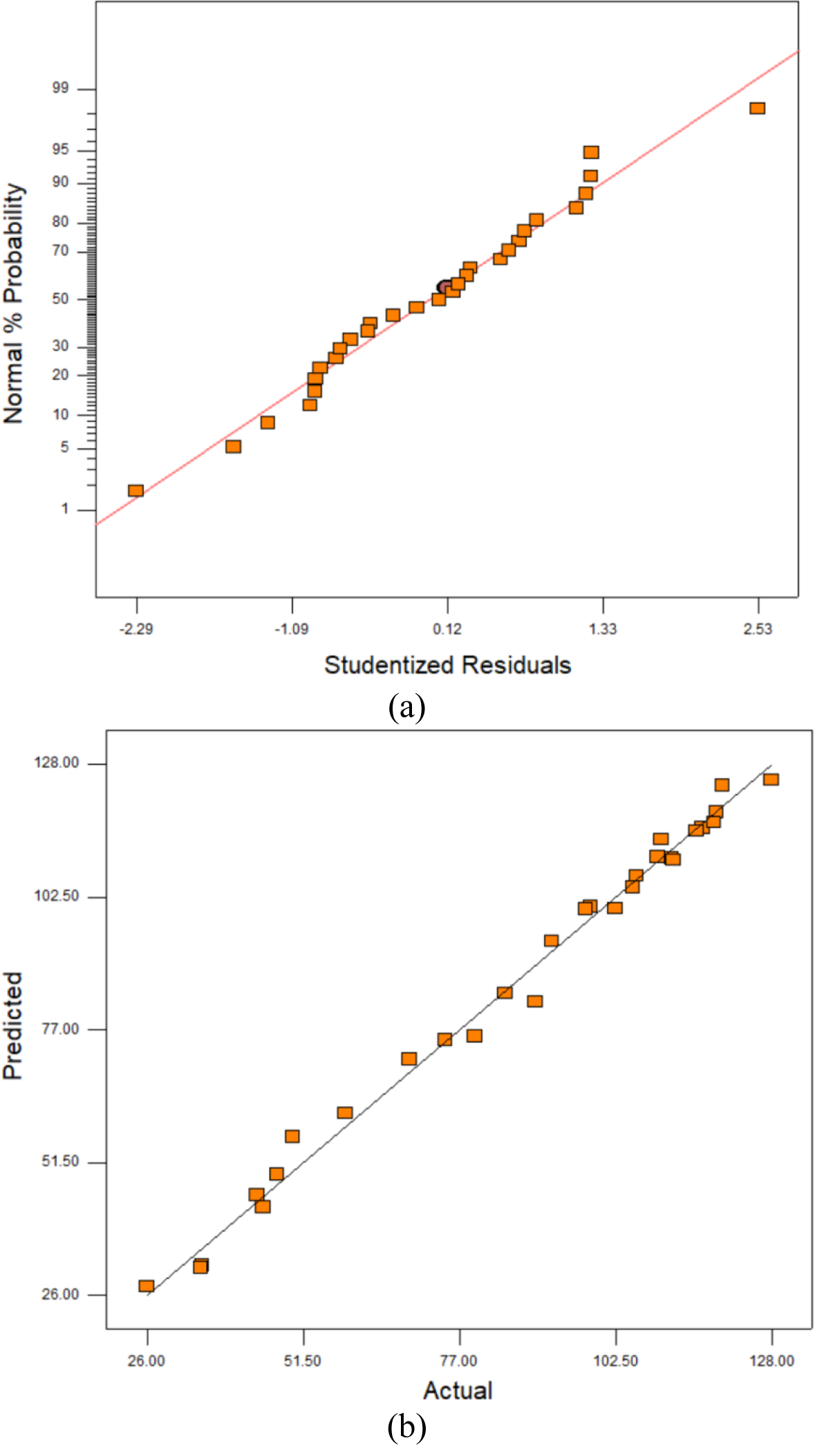
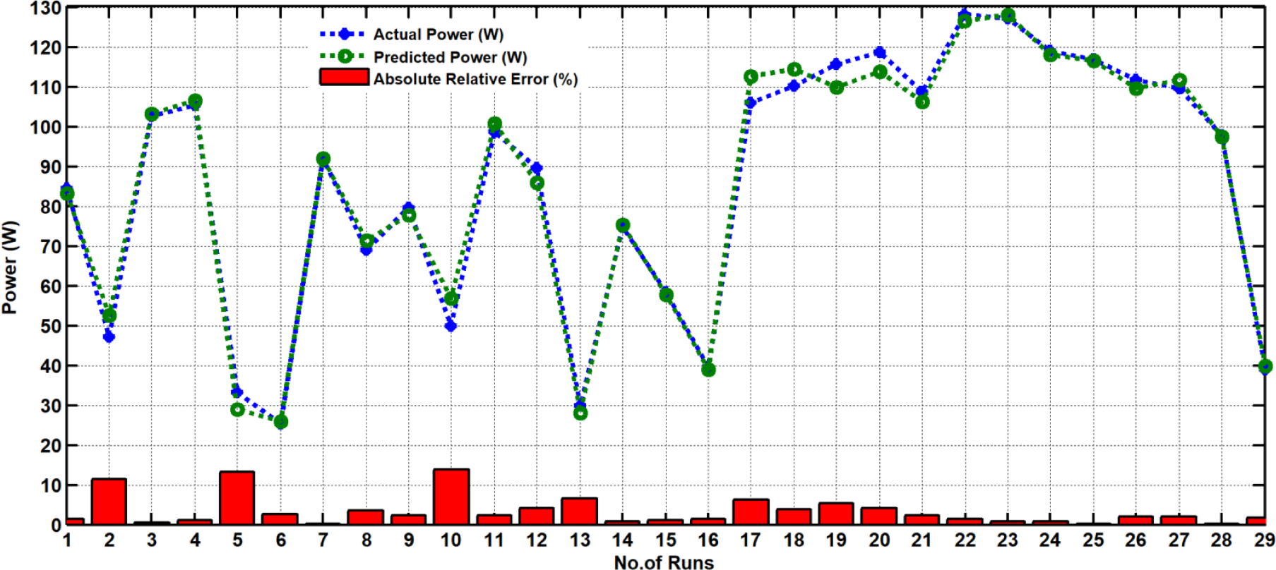
Figure 5 represents the diagnostic plots of generated power of RSM model. Figure 5a shows the normal plot of residual as confirmed by the normal probability. Figure 5b depicts the correlation plot between the predicted response and the experimental data. These plots are utilised to identify any potential discrepancies or divergences in the fit of the optimisation model to the experimental data. The points in these plots are distributed uniformly and followed a straight line. It indicates that the diagram assures the model developed. This suggests that the statistical model developed has captured the correlation among the three factors investigated in the production of power. Thus, it can be inferred that the chosen model is appropriate for accurately representing the relationship between the associated variables. Furthermore, Figure 5b displays a strong relationship between the experimental and predicted values of the generated power, indicating an excellent agreement between the two values. According to the results of the agreement between the actual data and model performance at a number of run, the convergence between the predicted power of PV module and the actual power is represented as shown in Figure 6. It is clear that the values of absolute relative deviation (ARD) are ranged between 0.2% to 13.3%.
Diagnostic plots of generated power for validation of RSM model (a) normal plot of residuals (b) actual and predicted plot
Plot of the ARD between the actual and predicted power values against to run number
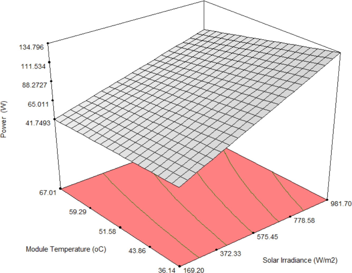
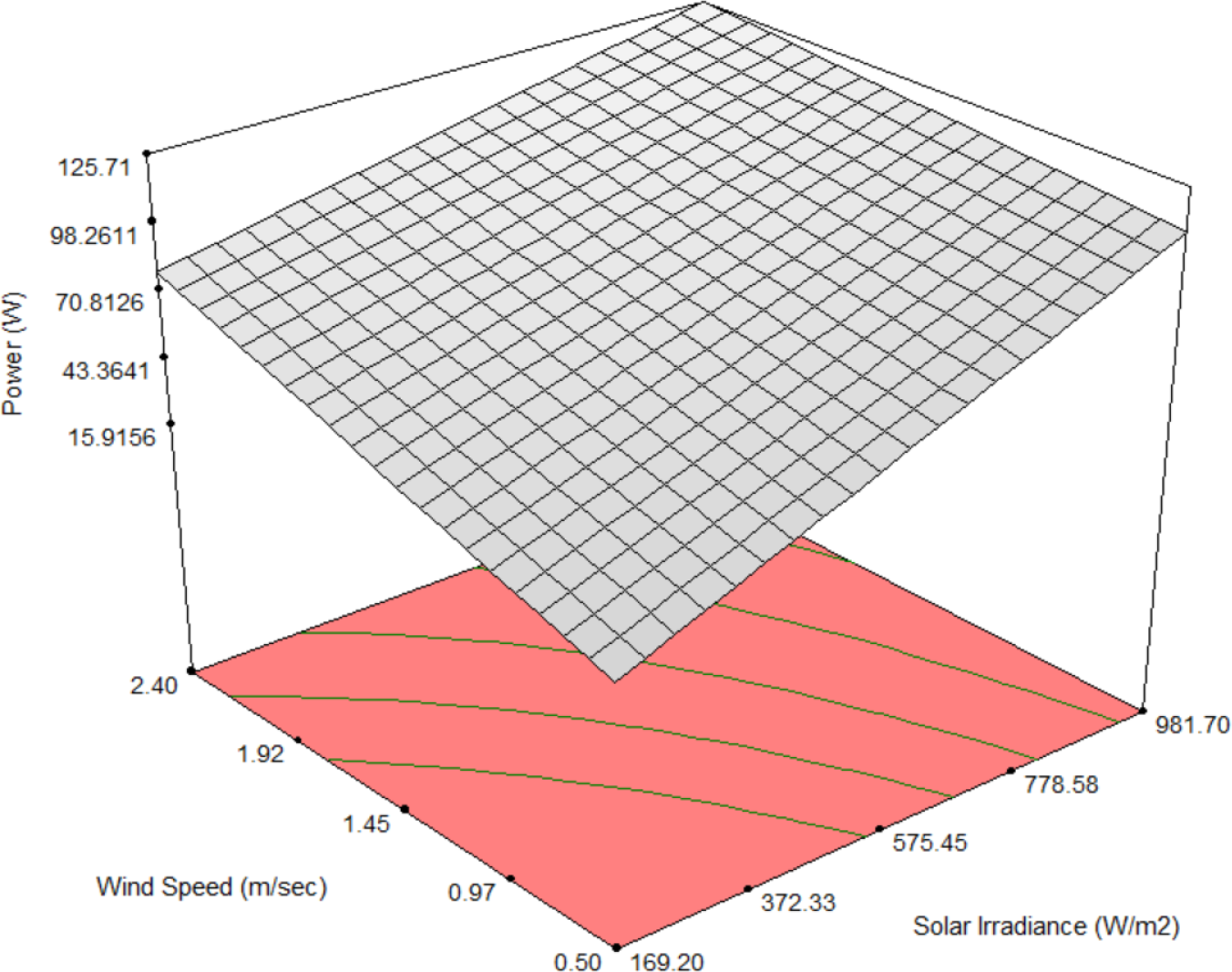
The three-dimensional (3D) surface plots of the generated power predicted by the model are plotted while utilising two experimental parameters and considering a fixed value of the third parameter as depicted in Figures 7, 8 and 9. These plots can aid to observe the trend of power generated (response) with respect to the increase or decrease in two operating parameters with a fixed third parameter. Figure 7 shows the power developed by the model for solar irradiance and module temperature at a constant wind speed 1.35 m/s. Specifically, the highest power of 134.7 W can be conducted at 981.7 W/m2 and 36.14 °C. Figure 8 shows the relationship between the solar irradiance, wind speed while considering a fixed module temperature of 51.58 °C. Herein, the maximum power of 125.71 W can be conducted at solar irradiance of 981.7 W/m2 and wind speed of 2.4 m/s. Figure 9 illustrates the response surface function developed by the model for module temperature and wind speed. The power presented a maximum of 103.44 W at 67.01 °C and 2.4 m/s with a constant solar irradiance of 575.45 W/m2.
3D graphical representations of the model for generated power against the module temperature and solar irradiance at wind speed 1.35 m/s
3D graphical representations of the model for generated power against the wind speed and solar irradiance at module temperature 51.58 °C
3D graphical representations of the model of generated power against the wind speed and module temperature at solar irradiance 575.45 W/m2
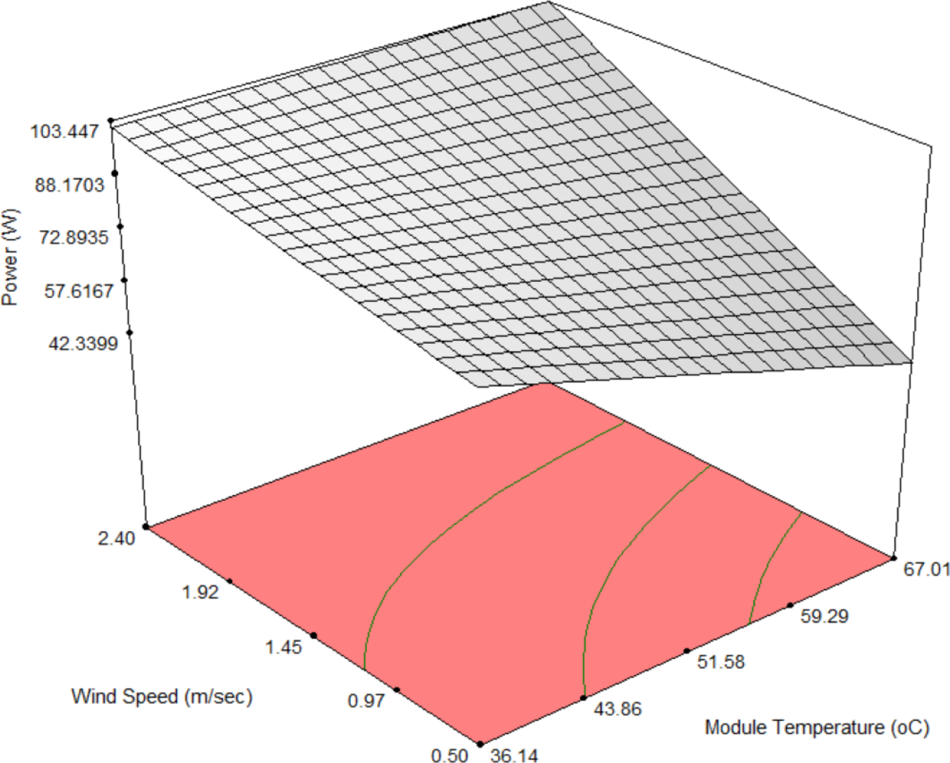
Table 4 summaries the values of generated power at the lowest and highest values of the third factor compared to the middle values that represented in Figure 6, 7 and 8. It is clear that an increase in the wind speed from 0.5 to 2.4 m/s would result in an increase in the generated power by 7.3%. However, increasing the module temperature from 36.1 to 67.01 °C would lead to a decrease of generated power by 13%. Also, an increase in the solar irradiance from 169.2 to 981.7 W would lead to an increase in the power by 25%.
A summary of generated power with the three levels of actual parameters
| Power (W) | Level of wind speed (m/s) | Level of module temperature (°C) | Level of solar irradiance (W/m2) | ||||||
|---|---|---|---|---|---|---|---|---|---|
| 0.5 | 1.35 | 2.4 | 36.1 | 51.58 | 67.01 | 169.2 | 575.45 | 981.7 | |
| Minimum | 79.7 | 101.5 | 117.1 | 131.9 | 107.4 | 80.43 | 14.3 | 42.33 | 78.16 |
| Maximum | 127.43 | 134.7 | 136.76 | 136.43 | 125.71 | 118.65 | 88.24 | 103.44 | 117.8 |
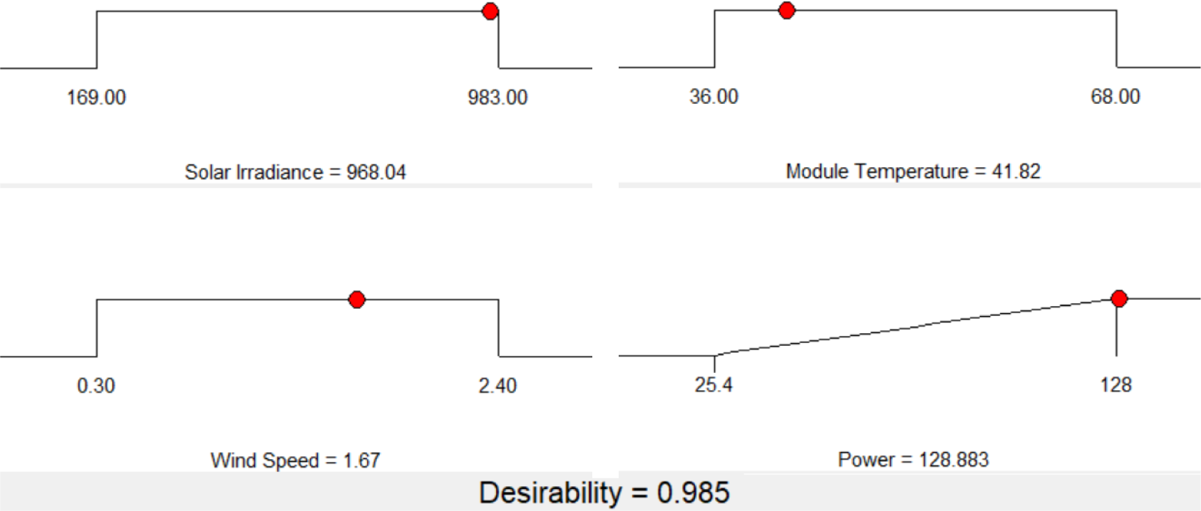
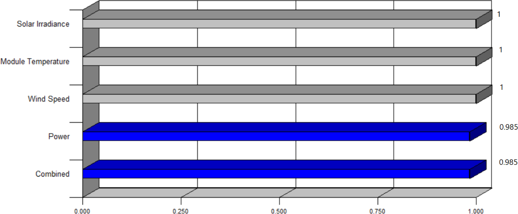
The results of RSM model optimisation are represented in Figures 10 and 11. As shown in Figure 10, the optimal conditions are solar irradiance of 968.04 W/m2, module temperature of 41.82 °C and wind speed of 1.67 m/s. Considering these optimal conditions, the maximum value of generated power is 128.883 W. This predicted value is in a perfect agreement with the experimental value of 127.1 W at the same conditions. Figure 11 shows the individual desirability values of control parameters, response variable, and combined optimisation with a combined desirability (D = 0.985). It is clear that the desirability function for control parameters (solar irradiance, module temperature and wind speed) is equal to 1 because they are set to be in a range of the optimisation. The response (generated power) optimised to be at a maximum level while the desirability function is obtained at 0.985.
Optimal conditions with the maximum value of power
Desirability values of control parameters, response variable, and combined optimisation
Multi regression statistical analysis was used to model and optimise the generated power of 165 WP of an individual PV module under different operation conditions of solar irradiance, module temperature and wind speed. The RSM model showed the relationship between the operations conditions and the generated power considered being linear. The predicted coefficient of determination R2 of 0.9845 is in reasonable agreement with the adjusted R2 of 0.9893. In addition, the results showed that the operation parameters have a noticeable impact on the generated power. Specifically, the solar irradiance and wind speed have positive effects on the generated power if compared to the module temperature. Thus, it can be inferred that the proposed model is appropriate for accurately representing the relationship between the associated variables. The maximum power of 128.883 W was attained for a set of optimal conditions of 968.04 W/m2 solar irradiance, 41.82 °C module temperature and 1.67 m/s wind speed, which designated by a maximum combined desirability function of D = 0.985. Moreover, the desirability function for control parameters (solar irradiance, module temperature and wind speed) is equal to 1 as they are set to be in a range of the optimisation.
This research is supported by Baqubah Technical Institute- Middle Technical University. The authors extend their thanks to the staff of institute, especially those working in the solar energy laboratory for their help.
| D | desirability function | [-] |
| k | number of independent variables | [-] |
| N | number of data points | [-] |
| P | generated power of PV module | [W] |
| R | coefficient of determination | [-] |
| S | solar irradiance | [W/m2] |
| TPV | temperature of PV module | [°C] |
| V | wind speed | [m/s] |
| X1,X2,…,Xk | independent variables | [-] |
| Y | response | [-] |
| Yi | actual value | [-] |
| predicted value | [-] | |
| mean value | [-] |
| β0 | constant | [-] |
| β1, β2, β3 | linear coefficients | [-] |
| β12, β13, β23 | interaction coefficients | [-] |
| ε | error of independent variables | [-] |
| MSE | Mean Square Error |
| RSS | Residual Sum of Squares |
| TSS | Total Sum of Squares |
| ARD | Absolute Relative Deviation |
- ,
Experimental investigation of soiling impact on PV module performance in Yanbu Al Sinaiyah, Saudi Arabia ,Renew. Energy , Vol. 216 ,pp 119117 , 2023, https://doi.org/https://doi.org/10.1016/j.renene.2023.119117 - ,
Influence of photovoltaic cell technologies and elevated temperature on photovoltaic system performance ,Ain Shams Eng. J. , Vol. 14 (7),pp 101984 , 2023, https://doi.org/https://doi.org/10.1016/j.asej.2022.101984 - ,
An Overview of Factors Affecting the Performance of Solar PV Systems ,Energy Scan , (27),pp 2–8 , 2017 - ,
Comparison of performance measurements of photovoltaic modules during winter months in Taxila, Pakistan ,Int. J. Photoenergy , Vol. 2014 , 2014, https://doi.org/https://doi.org/10.1155/2014/898414 - ,
The effect of environment on photovoltaic module efficiency ,Adv. Mater. Res. , Vol. 535–537 ,pp 1283–1286 , 2012, https://doi.org/https://doi.org/10.4028/www.scientific.net/AMR.535-537.1283 - ,
Effect of dust on the transparent cover of solar collectors ,Energy Convers. Manag. , Vol. 47 (18–19),pp 3192–3203 , 2006, https://doi.org/https://doi.org/10.1016/j.enconman.2006.02.014 - ,
Correlation between thicknesses of dust collected on photovoltaic module and difference in efficiencies in composite climate ,Int. J. Energy Environ. Eng. , Vol. 3 (1),pp 1–7 , 2012, https://doi.org/https://doi.org/10.1186/2251-6832-3-26 - ,
Modelling of conditions for accelerated lifetime testing of Humidity impact on PV-modules based on monitoring of climatic data ,Sol. Energy Mater. Sol. Cells , Vol. 99 ,pp 282–291 , 2012, https://doi.org/https://doi.org/10.1016/j.solmat.2011.12.011 - ,
Degradation analysis of installed solar photovoltaic (PV) modules under outdoor conditions in Ghana ,Energy Reports , Vol. 7 ,pp 6921–6931 , 2021, https://doi.org/https://doi.org/10.1016/j.egyr.2021.10.046 - ,
Variations of PV module parameters with irradiance and temperature ,Energy Procedia , Vol. 134 ,pp 276–285 , 2017, https://doi.org/https://doi.org/10.1016/j.egypro.2017.09.617 - ,
Impact of variation of solar irradiance and temperature on the inverter output for grid connected photo voltaic (PV) system at different climate conditions ,Mater. Today Proc. , Vol. 80 ,pp 2101–2108 , 2023, https://doi.org/https://doi.org/10.1016/j.matpr.2021.06.120 - ,
Temperature dependent photovoltaic (PV) efficiency and its effect on PV production in the world - A review ,Energy Procedia , Vol. 33 ,pp 311–321 , 2013, https://doi.org/https://doi.org/10.1016/j.egypro.2013.05.072 - ,
A Combined Experimental and Simulation Study on the Effects of Irradiance and Temperature on Photovoltaic Modules ,Energy Procedia , Vol. 75 ,pp 373–380 , 2015, https://doi.org/https://doi.org/10.1016/j.egypro.2015.07.393 - ,
Loss analysis and optimization of PV module components and design to achieve higher energy yield and longer service life in desert regions ,Appl. Energy , Vol. 280 ,pp 116028 , 2020, https://doi.org/https://doi.org/10.1016/j.apenergy.2020.116028 - ,
Experimental study on the impact of soiling on the modules temperature and performance of two different PV technologies under hot arid climate ,Heliyon , Vol. 8 (11),pp e11395 , 2022, https://doi.org/https://doi.org/10.1016/j.heliyon.2022.e11395 - ,
In-situ soiling evaluation and cleaning schedules optimization for several PV technologies under desert climate ,Renew. Energy , Vol. 224 ,pp 120167 , 20232024, https://doi.org/https://doi.org/10.1016/j.renene.2024.120167 - ,
Analysis of the dependence of the spectral factor of some PV technologies on the solar spectrum distribution ,Appl. Energy , Vol. 113 ,pp 302–309 , 2014, https://doi.org/https://doi.org/10.1016/j.apenergy.2013.07.044 - ,
Outdoor PV module performance under fluctuating irradiance conditions in tropical climates ,Energy Procedia , Vol. 33 ,pp 238–247 , 2013, https://doi.org/https://doi.org/10.1016/j.egypro.2013.05.064 - ,
Analysis of effects of solar irradiance, cell temperature and wind speed on photovoltaic systems performance ,Int. J. Energy Econ. Policy , Vol. 10 (1),pp 353–359 , 2020, https://doi.org/https://doi.org/10.32479/ijeep.8591 - ,
An overview of photovoltaic thermal combination (PV/T combi) technology ,Renew. Sustain. Energy Rev. , Vol. 38 ,pp 212–222 , 2014, https://doi.org/https://doi.org/10.1016/j.rser.2014.05.083 - ,
The value of day-ahead solar power forecasting improvement ,Sol. Energy , Vol. 129 ,pp 192–203 , 2016, https://doi.org/https://doi.org/10.1016/j.solener.2016.01.049 - ,
Short-term power forecasting system for photovoltaic plants ,Renew. Energy , Vol. 44 ,pp 311–317 , 2012, https://doi.org/https://doi.org/10.1016/j.renene.2012.01.108 - ,
Evaluating neural network and linear regression photovoltaic power forecasting models based on different input methods ,Energy Reports , Vol. 7 ,pp 7601–7614 , 2021, https://doi.org/https://doi.org/10.1016/j.egyr.2021.10.125 - ,
Validation of a multiple linear regression model for CIGSSe photovoltaic module performance and Pmpp prediction ,Sol. Energy , Vol. 208 ,pp 859–865 , 2020, https://doi.org/https://doi.org/10.1016/j.solener.2020.08.040 - ,
Online short-term solar power forecasting ,Sol. Energy , Vol. 83 (10),pp 1772–1783 , 2009, https://doi.org/https://doi.org/10.1016/j.solener.2009.05.016 - ,
Short term forecasting of solar radiation and power output of 89.6kWp solar PV power plant ,Mater. Today Proc. , Vol. 39 ,pp 1959–1969 , 2019, https://doi.org/https://doi.org/10.1016/j.matpr.2020.08.449 - ,
Prediction of the output power of photovoltaic module using artificial neural networks model with optimizing the neurons number ,Int. J. Renew. Energy Dev. , Vol. 12 (3),pp 478–487 , 2023, https://doi.org/https://doi.org/10.14710/ijred.2023.49972 - ,
Modeling and optimization i: Usability of response surface methodology ,J. Food Eng. , Vol. 78 (3),pp 836–845 , 2007, https://doi.org/https://doi.org/10.1016/j.jfoodeng.2005.11.024 - ,
Applications of Response Surface Methodology in the Food Industry Processes ,Food Bioprocess Technol. , Vol. 10 (3),pp 413–433 , 2017, https://doi.org/https://doi.org/10.1007/s11947-016-1855-2 - ,
Optimizing power consumption for CNC turned parts using response surface methodology and Taguchi’s technique-A comparative analysis ,J. Mater. Process. Technol. , Vol. 200 (1–3),pp 373–384 , 2008, https://doi.org/https://doi.org/10.1016/j.jmatprotec.2007.09.041 - ,
Response surface methodology for predicting the dimethylphenol removal from wastewater via reverse osmosis process ,Chem. Prod. Process Model. , Vol. 16 (3),pp 193–203 , 2021, https://doi.org/https://doi.org/10.1515/cppm-2020-0025 - ,
Experimental investigation on the effect of wind as a natural cooling agent for photovoltaic power plants in desert locations ,Case Stud. Therm. Eng. , Vol. 47 ,pp 103038 , 2023, https://doi.org/https://doi.org/10.1016/j.csite.2023.103038 - ,
Response surface methodology for anaerobic digestion of waste from poultry slaughterhouse: Optimization of load and hydraulic retention time ,Results Eng. , Vol. 18 ,pp 101215 , 2023, https://doi.org/https://doi.org/10.1016/j.rineng.2023.101215 - ,
A novel TOPSIS linear programming model based on response surface methodology for determining optimal mixture proportions of lightweight concrete blocks containing sugarcane bagasse ash ,Heliyon , Vol. 9 (7),pp e17755 , 2023, https://doi.org/https://doi.org/10.1016/j.heliyon.2023.e17755 - ,
Electrocoagulation of textile effluent: RSM and ANN modeling ,Int. J. Chem. React. Eng. , Vol. 7 , 2009, https://doi.org/https://doi.org/10.2202/1542-6580.1942 - ,
Response surface methodology (RSM) for optimizing engine performance and emissions fueled with biofuel: Review of RSM for sustainability energy transition ,Results Eng. , Vol. 18 ,pp 101213 , 2023, https://doi.org/https://doi.org/10.1016/j.rineng.2023.101213 - ,
Optimisation of lignin liquefaction with polyethylene glycol/ glycerol through response surface methodology modelling ,Ind. Crops Prod. , Vol. 198 , 2023, https://doi.org/https://doi.org/10.1016/j.indcrop.2023.116729 - ,
Evaluation of pistachio shells as solid wastes to produce activated carbon for CO2 capture: Isotherm, response surface methodology (RSM) and artificial neural network (ANN) modeling ,Curr. Res. Green Sustain. Chem. , Vol. 5 ,pp 100342 , 2022, https://doi.org/https://doi.org/10.1016/j.crgsc.2022.100342 - ,
Response surface optimization of electro-oxidation process for the treatment of C.I. Reactive Yellow 186 dye: reaction pathways ,Appl. Water Sci. , Vol. 7 (2),pp 637–652 , 2017, https://doi.org/https://doi.org/10.1007/s13201-015-0276-0 - ,
Measurement and Modeling of Gas Solubility and Literature Review of the Properties for the Carbon Dioxide-Water System ,Ind. Eng. Chem. Res. , Vol. 43 (7),pp 1794–1802 , 2004, https://doi.org/https://doi.org/10.1021/ie034232t


