


Maritime transport is currently one of the most important modes of transport and will remain like this for a long time. According to International Chamber of Shipping, around 90% of world trade is carried by the international shipping industry. Because of the competitive freight costs, shipping trade continues to expand and bring benefits to consumers around the world [1]. Maritime transport is the most cost-effective mode of transport. Significant advances in shipping technology and the ability of ships to transport an increased capacity of goods have given even more importance to this mode of transport [2].
The launch of container shipping is considered as one of the most significant progresses in the maritime cargo industry. Containerization have changed and revolutionised the way in which cargo is ferried and transported across the world, while increasing the safety and security of the transported cargo. Nowadays, many large shipping companies mainly deal with containerized cargo. Container ships are designed and constructed to transport huge amounts of various cargo. The cargo capacity of container ships is measured in terms of Twenty-foot Equivalent Unit (TEU), an inexact unit of cargo capacity based on the volume of a 20-foot-long (6.1 m) intermodal container. Due to their ability to transport high cargo capacities, some of the largest ships in the world are container ships [3]. The world’s largest container ship is OOCL Hong Kong, Ultra Large Container Vessel (ULCV), with a length of 399.87 m and cargo capacity of 21,413 TEU [4].
Driving such large ships requires a lot of power and consequently large fuel consumption, especially on large routes and heavier sea states. Reducing the fuel consumption and carbon emissions are two most important measures of shipping industry in order to minimize environmental impact, as emissions are in direct relation to fuel consumption. Even though maritime transport is the least polluting mode of transport per transported tonne of cargo, the International Maritime Organization (IMO) has proposed and implemented energy efficiency and Greenhouse Gas (GHG) regulations [5]. In recent years, shipping companies are faced with continuously increasing regulatory requirements. From January 1st, 2013 Ship Energy Efficiency Management Plan (SEEMP) and Energy Efficiency Design Index (EEDI) entered into force. More sea areas have been proclaimed as Emission Control Areas (ECA) in which stricter controls were established to minimize airborne emissions from ships [sulphur oxides (SOx), nitrogen oxides (NOx), Ozone Depleting Substances (ODS), Volatile Organic Compounds (VOC)] [6]. From January 1st, 2018 onwards, European Union (EU) has adopted a Regulation on monitoring, reporting and verification of carbon dioxide (CO2) emissions. The main purpose of this regulation is to promote the reduction of CO2 emissions by introducing a robust system of monitoring and reporting of data on annual fuel consumption, CO2 emissions and other energy efficiency-related parameters for ships above 5,000 gross tonnes, related to EU ports [7]. These regulatory measures will increase the cost of fuel and stimulate the achievement of greater energy efficiency, which is directly related to the total resistance of a ship.
The total resistance of a ship in waves consists of calm water resistance that is constant at a given constant speed and oscillating resistance due to motions of the ship, depending on the encounter wave frequency [8]. Planning a route in which greater sea states are avoided can have a large impact on fuel consumption. On the other hand, it should be taken into account that choosing larger routes with lower sea states over the minimum distance routes may increase the voyage time, and despite the reduction in fuel consumption and CO2 emission, the optimal environmental route solutions are not necessarily the optimal economic solutions at the same time [9]. Also, it may lead to risks of affecting the time delivery and the obligation of ship owners to ensure the voyages with reasonable dispatch and without changes in the usual route [10]. A way to reduce fuel consumption, and therefore fuel costs, is slow steaming [11]. The concept of slow steaming introduced for container shipping by Maersk Lines, has later been applied to other types of ships including tankers and dry bulk ships, whose operating speeds are traditionally low. Slow steaming has reduced the fuel consumption, which in turn has led to significant decrease in carbon emissions [12], [13]. When it comes to ship types, container ships are considered the main pollutant emitters causing up to 60% of total emissions in shipping [14]. Ammar [15] has investigated energy efficiency and cost efficiency of a ship sailing at the slow steaming speed in the Red Sea. The author showed that reducing the ship speed for 40% leads to a significant reduction in the CO2 emission and annual costs related to fuel consumption, and estimated the loss of profit per reduced knot.
Tezdogan et al. [16] have performed calculations of ship motions and added resistance in waves at the design and slow steaming speed for S175 container ship and the results showed a decrease of 53% in the vessel’s effective power and CO2 emission when the slow steaming approach was applied. The authors provided a valuable insight into the operational behaviour of the ship when not sailing at its design speed.
Since the influence of slow steaming on the overall voyage costs should be taken into account as well, Mallidis et al. [17] developed an analytical modelling methodology to assess the voyage costs due to an increased voyage time and the delays that may occur when sailing at slow steaming speed. Lee at al. [18] have proposed a model for the establishing the relation between the shipping time, fuel consumption and delivery reliability using set of industry data. The authors concluded that in order to keep the regular deliveries, additional vessels are required if slow steaming approach is applied. However, total savings in the fuel consumption are generally higher than the cost of operating additional vessels. Cepeda et al. [19] have investigated the benefits of slow steaming approach on the example of bulk carrier fleet. The authors pointed out higher efficiency of the fleet due to slow steaming, and the savings in fuel consumption and CO2 emission balanced the annual reduction in the transported cargo.
In this paper, the total resistance in waves, composed of calm water resistance and added resistance in waves, is calculated for a container ship at certain sea states for the North Atlantic using Computational Fluid Dynamics (CFD). The hull form of a typical container ship and a typical container ship trading route is chosen for the research at both the design and slow steaming speed. The obtained numerical results are validated against the experimental results available in the literature. For the purpose of spectral analysis, the significant wave height and zero crossing period are defined based on the wave statistics for the chosen route. The ratio of the fuel consumption for the slow steaming and the design speeds is calculated for the chosen route thus providing an insight into the potential savings in the fuel consumption, leading equivalently to CO2 emission reduction, on the realistic example.
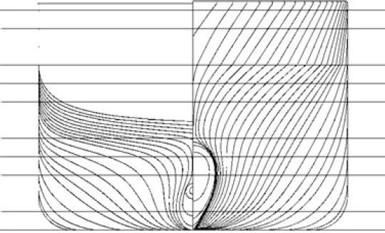
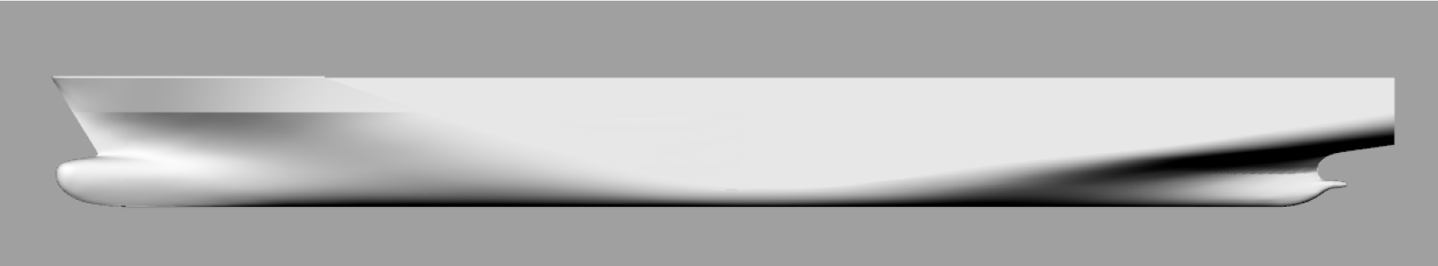
Numerical simulations of the flow around Kriso Container Ship (KCS) and KCS model are performed within commercial software packages HydroSTAR and STAR-CCM+ in order to determine the total resistance at certain sea states. KCS has a typical hull form of modern commercial container ships. Ship route analysed within this paper is common in today’s container transport. Therefore, the obtained results might point out the importance of speed reduction during the sail at certain sea states. The body plan of KCS is shown in Figure 1 and main particulars are given in Table 1. KCS 3D model is shown in Figure 2. Numerical simulations are performed for two Froude numbers (Fn), which correspond to the design and the slow steaming speeds, i.e., Fn = 0.26 and Fn = 0.195.
KCS body plan
Main particulars of KCS
| Main particulars | Model scale | Full scale |
|---|---|---|
| Length between perpendiculars (LPP) [m] | 7.2786 | 230 |
| Length of waterline (LWL) [m] | 7.3577 | 232.5 |
| Maximum beam of waterline (BWL) [m] | 1.0190 | 32.2 |
| Depth (D) [m] | 0.6013 | 19 |
| Draft (T) [m] | 0.3418 | 10.8 |
| Displacement volume (∇) [m3] | 1.6490 | 52,030 |
| Hull wetted surface area (SW) [m2] | 9.4379 | 9,424 |
| Block coefficient (CB) | 0.6505 | 0.6505 |
| Midship section coefficient (CM) | 0.9849 | 0.9849 |
| Longitudinal Centre of Buoyancy (LCB) (% LPP) from midship | −1.48 | −1.48 |
| Vertical Centre of Gravity (VCG) [m] | 0.2304 | 7.28 |
| Roll radius of gyration (kxx/B) | 0.40 | 0.40 |
| Pitch radius of gyration (kyy/LPP) | 0.25 | 0.25 |
| Yaw radius of gyration (kzz/LPP) | 0.25 | 0.25 |
| Density (ρ) [kg/m3] | 999.5 | 1,026 |
KCS 3D model
Numerical simulations of viscous flow around KCS model are performed within commercial software package STAR-CCM+, in order to determine the calm water resistance. Within numerical simulations, Reynolds Averaged Navier-Stokes (RANS) equations and averaged continuity equation are used as governing equations [20]:
(1)
(2)
where is the fluid density, is the averaged Cartesian components of the velocity vector, is the Reynolds stress tensor, is the mean pressure and is the mean viscous stress tensor defined by:
(3)
where μ is the dynamic viscosity.
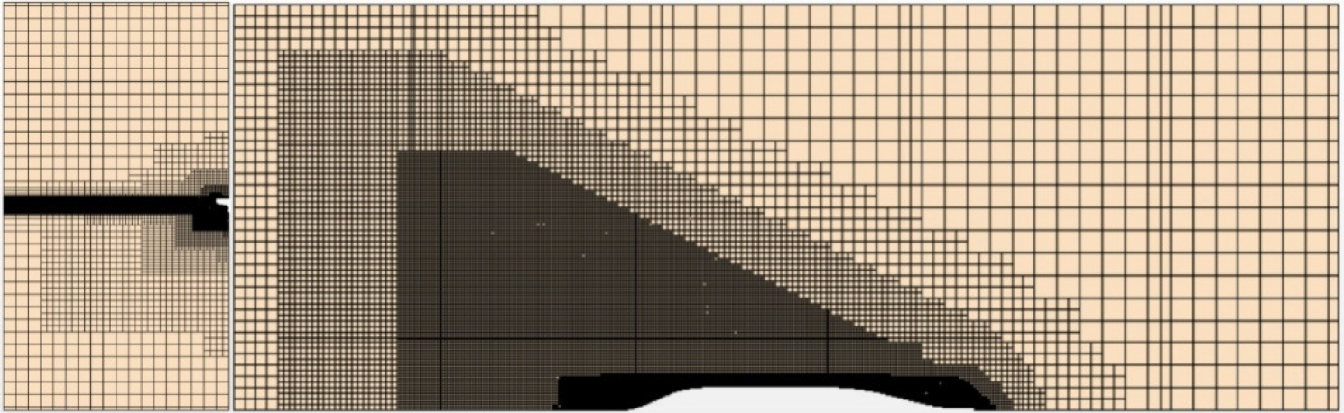
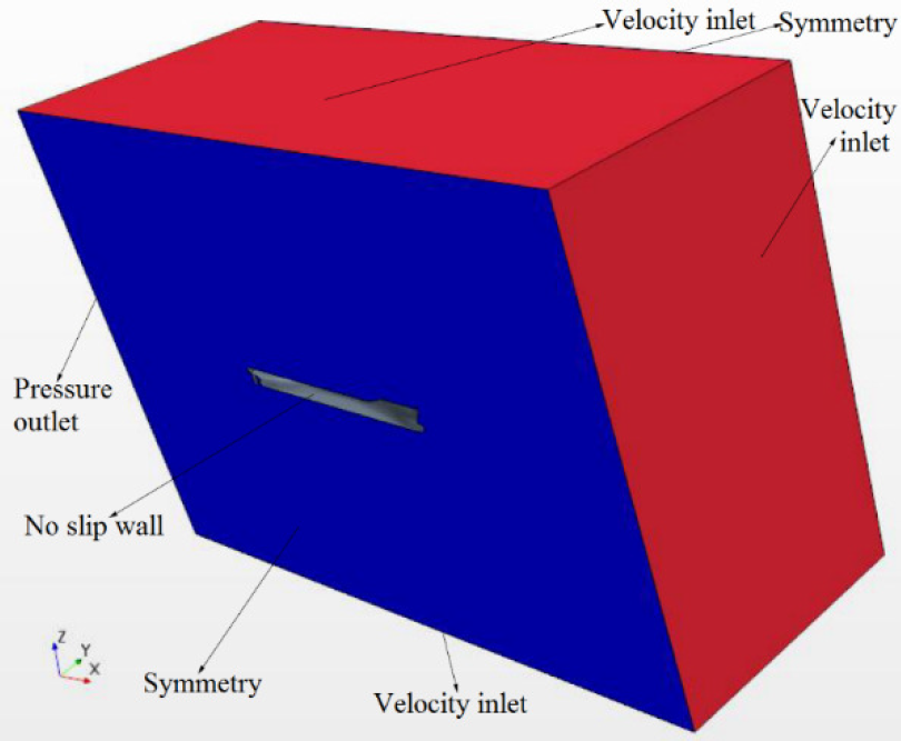
Realizible k-ε turbulence model [21], [22] is used for closing a set of eq. (1) and eq. (2). Volume of Fluid (VOF) method is used for tracking and locating the free surface. This method introduces a new parameter, the fraction of i-th fluid in the cell (αi). Thus eq. (1) and eq. (2) are solved only for one fluid and αi is determined using the averaged continuity equation. Finite Volume Method (FVM) is used for the discretization of eq. (1) and eq. (2), which are solved in segregated manner. First order Euler implicit scheme is used for temporal discretization, while second order upwind scheme is used for the discretization of convective terms. Computational domain is discretized with unstructured hexahedral mesh, which is refined in the region near the expected free surface, around the KCS model and for capturing the Kelvin wake (Figure 3). Six prism layers are made around the KCS model, in order to keep the non-dimensional wall distance (y +) value above 30. Thus, wall functions can be used, because the first cell from the wall is in the log-law region. Only half of domain is modelled, since symmetry condition is applied [23].
The structure of fine mesh, front view cross section (left) and top view cross section (right)
The domain boundaries are placed LPP away from the ship model in all directions. In order to prevent VOF wave reflection, VOF wave damping is applied using the damping function implemented in software package [24]. It should be noted that VOF wave damping length is set according to the ‘dvar’ function as follows:
(4)
where T is the period defined as ratio between LPP and KCS model speed.
Applied boundary conditions are shown in Figure 4. Numerical simulations are initialized with the initial velocity and pressure field. Time step used in this study is T/200, while the simulation is stopped after 20T.
Applied boundary conditions
The obtained results for the calm water resistance (RT) for KCS model are extrapolated to the full scale values using the extrapolation procedure described in Farkas et al. [24]. Index M represents physical property for model scale, and index S represents physical property for ship scale. The total resistance coefficient in calm water can be divided as follows:
(5)
where k is the form factor and for KCS is equal to k = 0.1 [2], CW is the wave resistance coefficient, assumed to be the same for model and ship (CWM = CWS) and CF is the frictional resistance coefficient defined according to the ITTC 1957 model-ship correlation line:
(6)
where Rn is the Reynolds number.
In order to obtain CTS, firstly CW has to be determined as follows:
(7)
where CTM is calculated according to:
(8)
where RTM is the calm water resistance of KCS model obtained from numerical simulation, ρM is the water density and vM is the KCS model speed.
After CW is determined, CFS is calculated according to the eq. (6) and then CTS can be easily determined utilizing eq. (5). The calm water resistance of full scale ship can be calculated according to the following equation:
(9)
where ρS is the sea water density.
The added resistance of a ship in waves is one of the main causes of an involuntary speed reduction and an increase of the fuel consumption. Considering its direct effect on CO2 emission, it is very important to estimate an increase of the total resistance due to waves especially at heavier sea states. In severe sea states, ship may experience an increase in resistance larger than the one that is commonly taken into account as a percentage of the calm water resistance known as Sea Margin (SM).
The added resistance in waves is the second order wave force and is considered to be independent on the calm water resistance. Viscous part of the added resistance in waves is negligible, thus it is justified to calculate the ship added resistance using numerical tools based on the potential flow of fairly perfect fluid. Despite the fact that numerical tools based on the viscous flow theory are proven to be more accurate and sophisticated than the ones based on the potential flow theory, the latter ones are still widely used in hydrodynamic calculations due to their robustness, low required computational time and reliability [25].
In this paper, the added resistance of KCS container ship is determined utilizing the commercial software package HydroSTAR v.7.3 [26], based on the potential flow theory at regular head waves. Ship advancing speed is taken into account through the encounter frequency of incoming waves. The obtained results are validated, i.e., compared with the experimental data available in the literature.
Panel method within software package HydroSTAR provides the first order wave radiation and diffraction solution as well as the solution of the second-order wave loads. The velocity potential, used to describe the flow around ship hull, satisfies Laplace equation in the entire computational domain and consists of incoming wave potential ΦI and perturbation potential ΦP due to presence of the ship. Perturbation potential can be decomposed on its diffraction and radiation part.
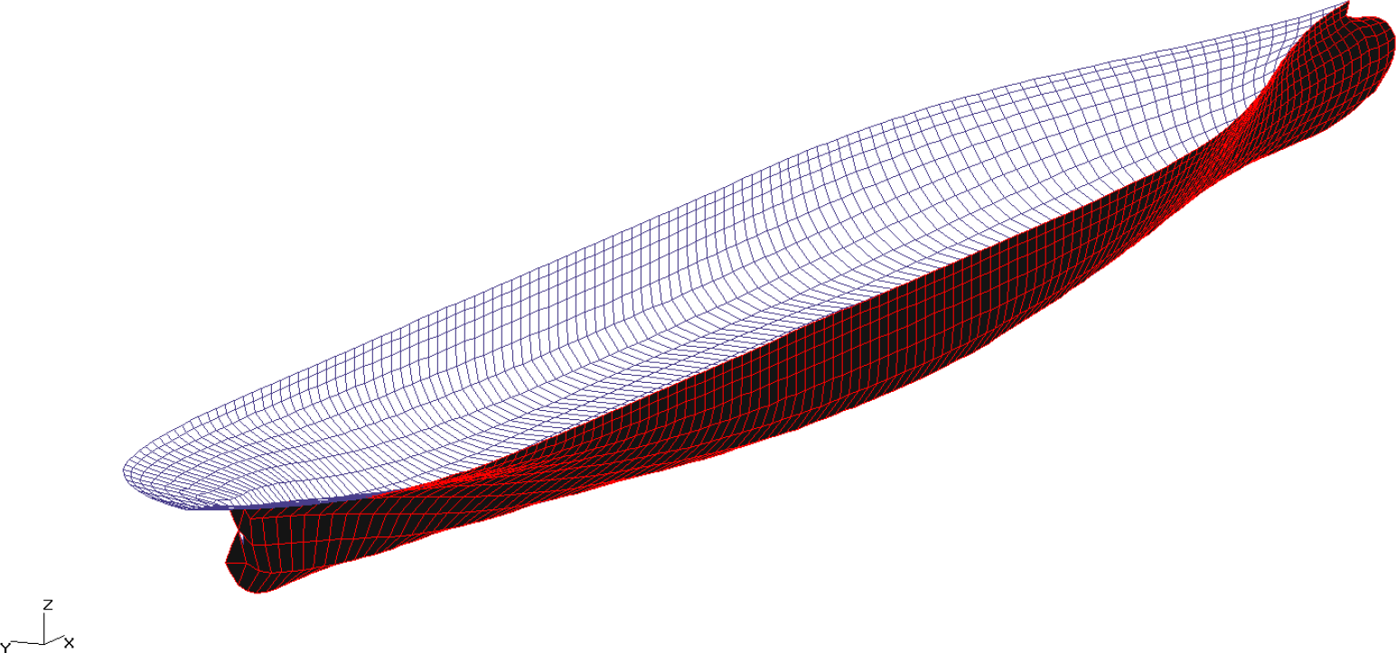
In panel method, body is discretized using flat panels with sources and dipoles of constant strength on each panel. Integral equations, known as Boundary Integral Equations (BIE), are then solved for the unknown strength of sources and dipoles, based on so called Green function. Hull of the KCS container ship as well as the interior free surface of the hull are discretized using quadrilateral panels as can be seen in Figure 5.
Panel model of the KCS container ship
In the frequency domain the velocity potential can be expressed as the real part of complex function . Green function as the fundamental solution of Laplace equation is formulated in order to satisfy boundary condition on the linearized free surface, on the seabed and hull, and radiation condition in the far field as follows:
(10)
(11)
(12)
(13)
where k is the wave number, n is the unit surface normal of boundary element and is oriented towards fluid and vn is the normal velocity on the boundary element. Radiation condition, which requires that the velocity potential disappears in the infinite boundary around the ship hull, is automatically satisfied when Kelvin type Green function is used.
With known velocity potential, pressure on each panel can be calculated with modified Bernoulli equation. Forces and moments acting on ship hull are then calculated by the direct pressure integration along the wetted surface S and waterline L in their mean position, by the so-called near-field formulation as follows:
(14)
where ωi is the frequency of incoming wave, ϕ is the first order velocity potential, ϕn is the normal derivative of first order velocity potential on hull surface, ϕ* is the complex conjugate of first order velocity potential and is the complex conjugate of normal derivative of first order velocity potential on hull surface.
Since the added resistance in waves is determined through the Quadratic Transfer Function (QTF) approximated by zeroth-term only, the obtained force is a constant value at each given frequency of incoming wave.
In order to determine the ship response at irregular waves related to actual sea states, the wave energy density spectrum is used. It represents the energy of particular harmonic component of the irregular wave.
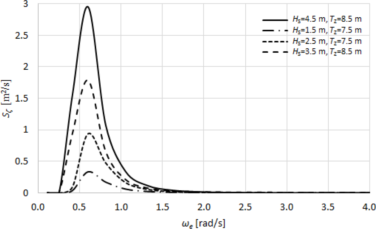
In this paper, the ship added resistance at actual sea state corresponding to the North Atlantic is obtained using the Bretschneider or two-parameter Pierson-Moskowitz sea spectrum recommended for the North Atlantic. One parameter of the spectrum is significant wave height HS, i.e., mean wave height (trough to crest) of the highest third of the all wave heights and second parameter is zero crossing period Tz, i.e., mean time interval between upward or downward zero crossings of a wave. The Bretschneider wave spectrum is defined by the following expression:
(15)
where ω is the wave frequency.
The spectral function of the ship added resistance in waves is obtained by multiplying drift force at certain frequency and the corresponding ordinate of the wave spectrum. The first spectral moment, i.e., integral of the spectral function, is obtained using the trapezoidal rule of integration. The mean value of the added resistance at the defined sea state is thus based on the absolute values of the drift forces and the contribution of wave energy over the whole frequency range of interest. It should be noted that mean added resistance of ship advancing in waves is calculated based on the encounter frequency of the incoming waves as follows [27]:
(16)
where stands for the drift force at certain wave frequency obtained using hydrodynamic software HydroSTAR [26], is the unit wave amplitude and ωe is the encounter frequency defined as follows:
(17)
where v is the ship advancing speed and β is the wave heading.
The verification study is made for grid size, as it is the main source of numerical uncertainty. Within numerical simulations of viscous flow around the hull, grids are refined uniformly. Thus, the obtained number of cells for coarse mesh is around 0.5 M, for medium mesh 1 M and for fine mesh 2 M. The numerical uncertainty is estimated according to Grid Convergence Index (GCI) method, which is relied on Richardson extrapolation.
The apparent order of method is given with:
(18)
where r21 and r32 are equal to 1.26, ε32 = ϕ3 − ϕ2, ε21 = ϕ2 – ϕ1, and ϕi is the solution obtained with i-th grid and q(pa) is defined as:
(19)
(20)
The extrapolated solution is calculated according to:
(21)
while the approximate and extrapolated errors are calculated as follows:
(22)
(23)
Finally, the grid convergence index for fine input parameter is assessed with:
(24)
In this section, the obtained numerical results for the calm water resistance as well as the added resistance in waves are presented. Furthermore, the benefit of speed reduction is shown in terms of fuel consumption.
Verification study is carried out at Fn = 0.260 and the obtained results are shown in Table 2. As can be seen, the obtained numerical uncertainty is equal to 2.14%. It should be noted that the fine mesh is used for numerical simulation at Fn = 0.195.
Validation of the calm water resistance coefficient
| ϕ3 [N] | ϕ2 [N] | ϕ1 [N] | pa | [N] | [%] |
|---|---|---|---|---|---|
| 82.492 | 82.946 | 83.611 | 1.652 | 85.042 | 2.139 |
Numerical simulations of viscous flow around KCS model are performed and the obtained results are validated against the experimental results available in the literature [28] (Table 3). The relative deviation between the numerical and experimental results is calculated as follows:
(25)
Validation of the calm water resistance coefficient
| Fn | 103 CT,EXP | 103 CT,CFD | RD [%] |
|---|---|---|---|
| 0.195 | 3.475 | 3.399 | −2.187 |
| 0.260 | 3.711 | 3.628 | −2.236 |
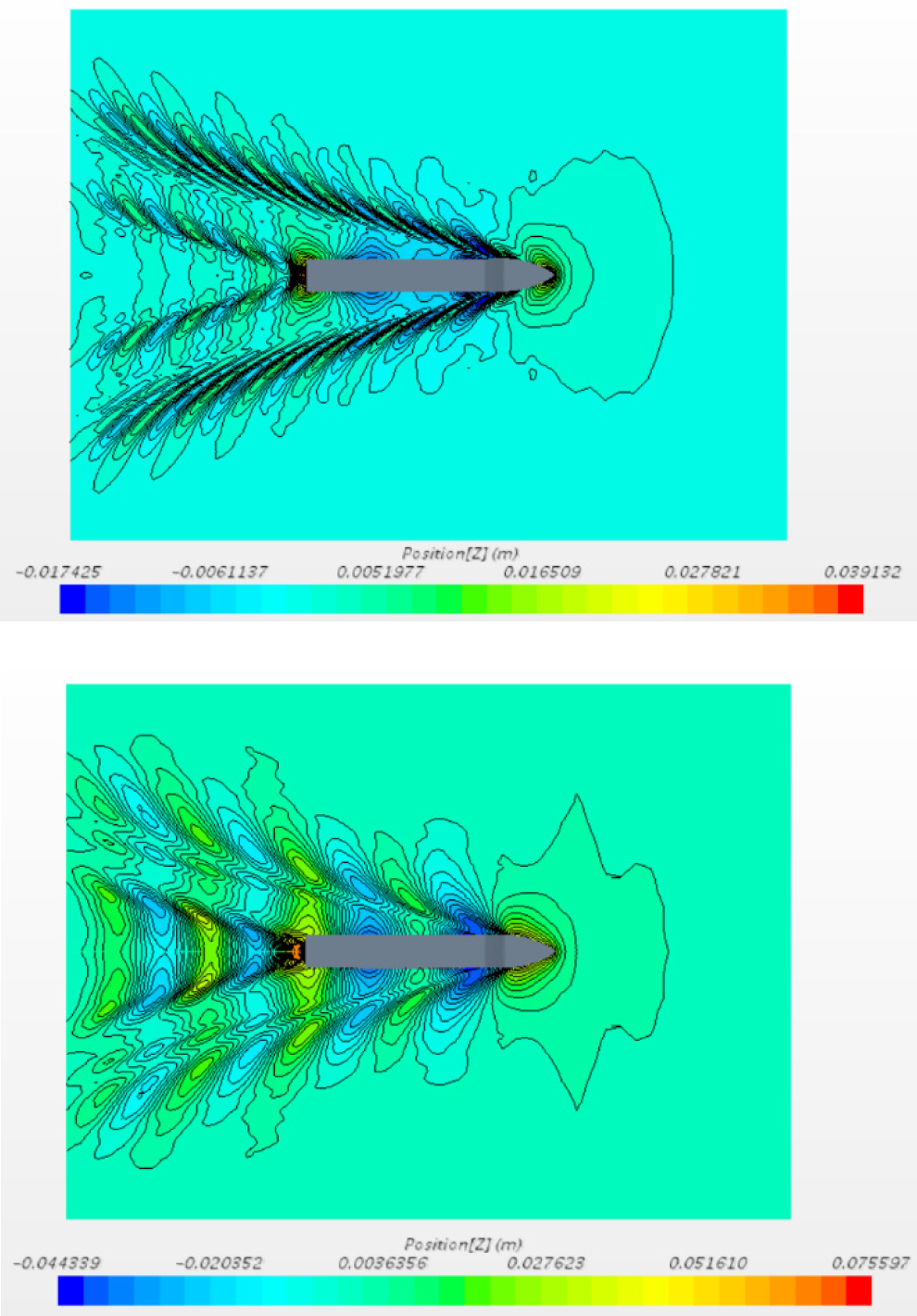
The wave patterns obtained with fine mesh for two Fn are shown in Figure 6.
Wave patterns for Fn = 0.195 (top) and Fn = 0.260 (bottom)
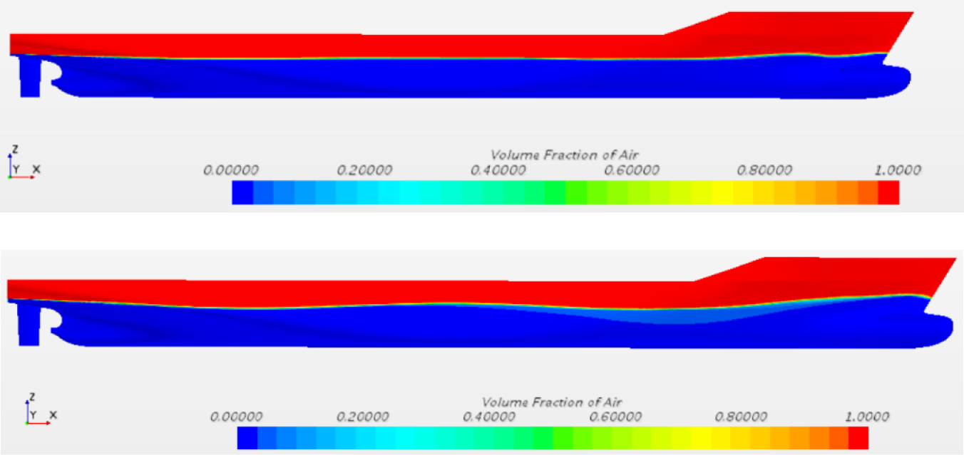
The wave profiles on the KCS model obtained utilizing fine mesh for two Fn are shown in Figure 7. It can be seen that the bow and stern wave systems begin with a wave crest, while the systems of bow and stern shoulders begin with a wave through.
Wave profiles for Fn = 0.195 (top) and Fn = 0.260 (bottom)
The obtained values of the calm water resistance for KCS model are extrapolated according to the procedure described in section Methodology. For Fn = 0.260, which corresponds to the design speed VD = 24 knots, the calm water resistance is equal to 1,471 kN. For Fn = 0.195, which corresponds to the slow steaming speed VS = 18 knots, the calm water resistance is equal to 686 kN.
The results for the added resistance in regular waves of unit amplitude are validated against the experimental data available in Simonsen et al. [29] at Fn = 0.260 (Table 4).
Validation of non-dimensional value of the added resistance in waves
| ω [rad/s] | RD [%] | ||
|---|---|---|---|
| 0.4263 | 5.750 | 6.245 | 8.611 |
| 0.4504 | 8.717 | 9.026 | 3.543 |
| 0.4896 | 11.155 | 10.920 | −2.106 |
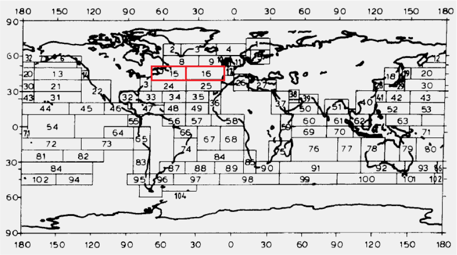
Spectral analysis, as described in section Methods, is performed in order to obtain the mean added resistance for certain sea states. Results calculated for regular waves of unit amplitude in the defined frequency range for two Fn are used for spectral analysis. In order to simulate real sailing conditions of container ships, the common container ship route Southampton-Boston is chosen. The route length is equal to 3,000 nautical miles. Significant wave height as well as zero crossing period which define certain sea state, are chosen based on Global Wave Statistics [30].
The chosen route pass through sea areas 15 and 16 in the North Atlantic (Figure 8).
Considered sea areas in the North Atlantic
Bretschneider spectrum for certain sea states is shown in Figure 9. It can be seen that most of the spectral energy is contained in waves of lower frequencies.
Bretschneider spectrum for certain sea states
Under the assumption of constant specific fuel consumption and propulsive efficiency, the ratio of the fuel consumption per route for the slow steaming and the design speeds BS/BD is calculated as follows:
(26)
where RTW,D is the sum of the calm water resistance and the added resistance in waves at the design speed, RTW,S is the sum of the calm water resistance and the added resistance in waves at the slow steaming speed, tD is the route duration at the design speed and tS is the route duration at the slow steaming speed.
The mean value of the added resistance in waves, the total resistance in waves and the effective power for certain sea states for Fn = 0.260, which corresponds to the design speed and Fn = 0.195, which corresponds to the slow steaming speed are calculated and given in Tables 5 and 6, respectively. Furthermore, the ratio of the fuel consumption per route for the slow steaming and the design speeds BS/BD is given in Table 6. The relation between the effective power and certain sea state for two mentioned speeds is shown in Figure 10.
The obtained results for the design speed
| No. | HS [m] | Tz [s] | RAW [kN] | RTW [kN] | PE [kW] |
|---|---|---|---|---|---|
| 1 | 1.5 | 7.5 | 61.51 | 1,532.51 | 18,919.78 |
| 2 | 2.5 | 7.5 | 170.87 | 1,641.87 | 20,269.82 |
| 3 | 3.5 | 8.5 | 264.82 | 1,735.82 | 21,429.72 |
| 4 | 4.5 | 8.5 | 437.76 | 1,908.76 | 23,564.80 |
The obtained results for the slow steaming speed
| No. | HS [m] | Tz [s] | RAW [kN] | RTW [kN] | PE [kW] | BS/BD [%] |
|---|---|---|---|---|---|---|
| 1 | 1.5 | 7.5 | 53.08 | 739.08 | 6,843.31 | 48.23 |
| 2 | 2.5 | 7.5 | 147.45 | 833.45 | 7,717.09 | 50.76 |
| 3 | 3.5 | 8.5 | 235.53 | 921.53 | 8,532.67 | 53.09 |
| 4 | 4.5 | 8.5 | 389.35 | 1,075.35 | 9,956.90 | 56.34 |
Effective power for certain sea states
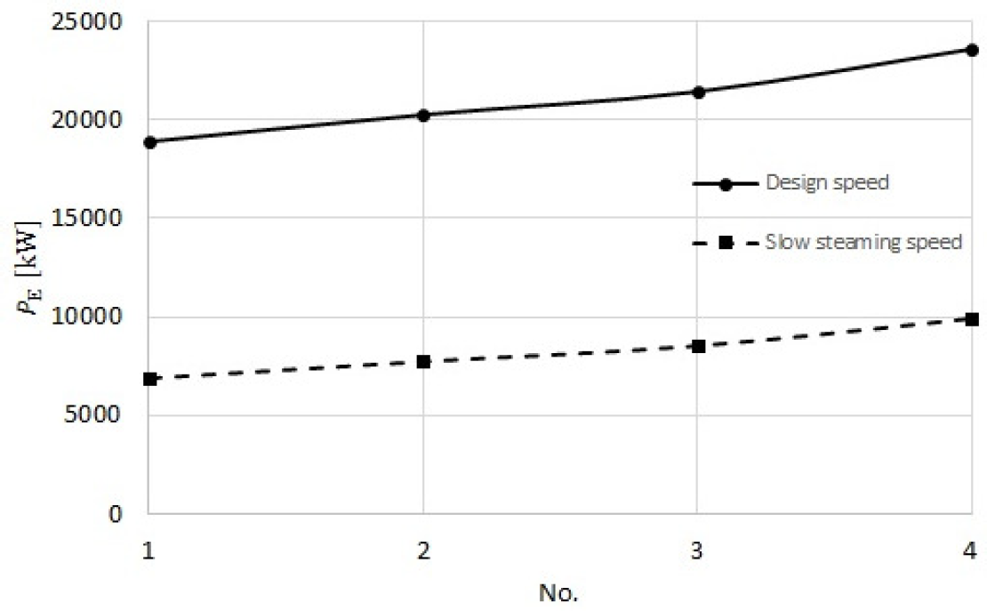
It can be seen from Figure 10 that the effective power increases at higher sea states. For lower sea states, the portion of the calm water resistance in total resistance in waves is larger than for higher sea states. It should be noted that for the design speed the calm water resistance is significantly higher than the calm water resistance for the slow steaming speed. Thus, the obtained percentage savings in fuel consumption at heavier sea states are lower compared to ones for lower sea states (Figure 11).
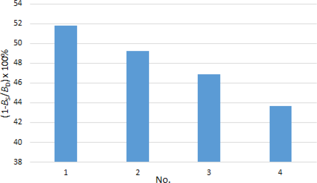
For example, for the heaviest sea state considered, the calculated ratio BS/BD is equal to 0.563. Therefore, when the design speed is reduced to the slow steaming speed, the fuel consumption per route decreases for 43.7%. However, it should be noted that the route duration for the slow steaming speed is 33.3% larger compared to the route duration for the design speed.
Estimation of the percentage savings in fuel consumption for certain sea states
The total resistance in waves for a typical container ship was calculated at the design and the slow steaming speeds. The calm water resistance was calculated utilizing CFD based on viscous flow and the added resistance in waves was calculated using CFD based on potential flow. The obtained numerical results show satisfactory agreement with the experimental results available in the literature. The calm water resistance was determined for KCS model and the obtained results are extrapolated to full scale values. The added resistance in waves was calculated at regular waves of unit amplitude. Spectral analysis for certain sea states corresponding to the North Atlantic was performed based on the Bretschneider spectrum, defined by significant wave height and zero crossing period. The ratio of fuel consumption at the slow steaming and the design speeds was determined as well. The results show the importance of the speed reduction in terms of fuel consumption per route. Under the assumption of complete combustion, the decrease of fuel consumption is equivalent to the decrease of CO2 emission, what is of great importance from the environmental point of view. However, it should be noted that the route duration at the slow steaming speed is larger compared to one at the design speed, which causes larger route costs as well as lower number of routes per year, i.e., lower profit per year.
For that reason, the part of future work will include economic analysis that will clarify weather savings in fuel at reduced ship speed are economically justified regarding higher ship expenses and lower profit.
- , , 2019
- ,
Predicting the Effect of Biofouling on Ship Resistance using CFD ,Applied Ocean Research , Vol. 62 ,pp 100-118 , 2017, https://doi.org/https://doi.org/10.1016/j.apor.2016.12.003 - , , 2019
- , , 2019
- , Implications of the United Nations Convention on the Law of the Sea for the International Maritime Organization, Study by the Secretariat of the International Maritime Organization (IMO), 2014
- , Energy Management Study, 20152019
- , , 2019
- ,
Added Resistance in Waves of Intact and Damaged Ship in the Adriatic Sea ,Brodogradnja , Vol. 66 (2),pp 1-14 , 2015 - ,
Ship Speed Optimization: Concepts, Models and Combined Speed-routing Scenarios ,Transportation Research Part C , Vol. 44 ,pp 52-69 , 2014, https://doi.org/https://doi.org/10.1016/j.trc.2014.03.001 - ,
An utility-based Decision Support Sustainability Model in Slow Steaming Maritime Operations ,Transportation Research Part E: Logistics and Transportation Review , Vol. 78 ,pp 57-69 , 2015, https://doi.org/https://doi.org/10.1016/j.tre.2015.01.013 - ,
Full-scale Unsteady RANS CFD Simulations of Ship Behavior and Performance in Head Seas due to Slow Steaming ,Ocean Engineering , Vol. 97 ,pp 186-206 , 2015, https://doi.org/https://doi.org/10.1016/j.oceaneng.2015.01.011 - , , 2019
- ,
How to Decarbonise International Shipping: Options for Fuels, Technologies and Policies ,Energy Conversion and Management , Vol. 182 ,pp 72-88 , 2019, https://doi.org/https://doi.org/10.1016/j.enconman.2018.12.080 - ,
The activity-based Methodology to Assess Ship Emissions ‒ A Review ,Environmental Pollution , Vol. 231 ,pp 87-103 , 2017, https://doi.org/https://doi.org/10.1016/j.envpol.2017.07.099, Part 1 - , Energy- and Cost-efficiency Analysis of Greenhouse Gas Emission Reduction using Slow Steaming of Ships: Case Study RO-RO Cargo Vessel, Vol. 13, No. 8, pp 868-876, Ships Offshore Structures, 2018
- ,
Assessing the Impact of a Slow Steaming Approach on Reducing the Fuel Consumption of a Containership Advancing in Head Seas ,Transportation Research Procedia , Vol. 14 ,pp 1659-1668 , 2016, https://doi.org/https://doi.org/10.1016/j.trpro.2016.05.131 - ,
The Impact of Slow Steaming on the Carriers’ and Shippers’ Costs: The Case of a Global Logistics Network ,Transportation Research Part E , Vol. 111 ,pp 18-39 , 2018, https://doi.org/https://doi.org/10.1016/j.tre.2017.12.008 - ,
The Impact of Slow Ocean Steaming on Delivery Reliability and Fuel Consumption ,Transportation Research Part E , Vol. 76 ,pp 176-190 , 2015, https://doi.org/https://doi.org/10.1016/j.tre.2015.02.004 - ,
Effects of Slow Steaming Strategies on a Ship Fleet ,Marine Systems & Ocean Technology , Vol. 12 ,pp 178-186 , 2017, https://doi.org/https://doi.org/10.1007/s40868-017-0033-3 - , , Computational Methods for Fluid Dynamics, 2012
- , STAR-CCM+ User Guide, 2017
- ,
Free Surface Flow Simulation Around an Appended Ship Hull ,Brodogradnja , Vol. 69 (3),pp 25-41 , 2018, https://doi.org/https://doi.org/10.21278/brod69302 - , Simulation of Flow Around KCS-hull, Proceedings from Gothenburg 2010 ‒ A Workshop on Numerical Ship Hydrodynamics, 2010
- ,
Numerical Simulation of Viscous Flow Around a Tanker Model ,Brodogradnja , Vol. 68 (2),pp 109-125 , 2017, https://doi.org/https://doi.org/10.21278/brod68208 - ,
Added Resistance of Ships in Waves ,Ship Technology Research-Schiffstechnik , Vol. 62 (1),pp 2-13 , 2015, https://doi.org/https://doi.org/10.1179/0937725515Z.0000000001 - , Bureau Veritas, 2016
- , , Offshore Hydromechanics, 2001
- , , 2019
- ,
EFD and CFD for KCS Heaving and Pitching in Regular Head Waves ,Journal of Marine Science and Technology , Vol. 18 (4),pp 435-459 , 2013, https://doi.org/https://doi.org/10.1007/s00773-013-0219-0 - , , Global Wave Statistics, 1986