


Water demand is anticipated to immensely increase over the coming years, particularly for the industrial sector [1]. In high-income countries, 70% of wastewater undergoes treatment. However, the statistics are different in low-income countries, where only 8% of wastewater is treated. On average, 80% of global generated wastewater are not appropriately treated [2].
These concerns have driven efforts towards extensive PI methodologies that have been developed for water minimisation over the past years. Starting from the works of Wang and Smith [3], water and wastewater minimisation via water integration have been widely extended to Total Site (TS) water minimisation [4].
Water Integration at TS is also known as Interplant Water Integration (IPWI). Olesen and Polley [5] work on IPWI considering the layout of plant and piping is one of the earliest work in this field. Keckler and Allen [6] developed mathematical optimisation to locate the potentials of water reuse in industrial parks. New IPWI configuration incorporating internal water main to collect water sources at a specific range of concentrations before utilised is proposed by Feng and Seider [7]. Liao et al. [8] combine pinch analysis based method with mathematical optimisation to solve the multiperiod problem in IPWI considering operational flexibility and cost of piping. Cross-plant pipelines and centralised utility hub were used to study direct and indirect IPWI integration [9]. Water cascade analysis [10] was initially developed for a single water network and later extended by Foo [11] for IPWI integration. Bandyopadhyay et al. [12] developed algorithmic decomposition technique on segregated targeting problems. Chen et al. [13] proposed a new technique of IPWI via central and decentralised water mains (reservoir). Sahu and Bandyopadhyay [14] developed a rigorous algebraic algorithm for IPWI with two plants. Boix et al. [15] identify the suitability of adding regeneration unit for IPWI with three plants. Alnouri et al. [16] proposed pipeline branching options for direct IPWI. Jia et al. [17] studies IPWI by considering water supply constraint with differential water price. Alnouri et al. [18] extended IPWI methodology with pipeline branching options by adding regeneration and wastewater treatment. Liu et al. [19] identify the possibilities of mixing in IPWI. Recently, Alnouri et al. [20] studied on zero liquid discharge (central and decentralised) IPWI.
Fadzil et al. [21] proposed an innovative methodology of Total Site Centralised Water Integration (TS-CWI) using Centralised Water Reuse Header (CWRH). The methodology offers a more straightforward and practical interplant water network for implementation. The third-party owning the CWRH system provides an opportunity for industries to make profits by selling their water sources to the CWRH while buying inexpensive low-grade water for reusing purposes since not every process needs clean freshwater to operate. The owner of the system also responsible for protecting confidential data and information from various companies.
However, there is a concern about how the number of CWRH affecting consumer and operator. Increasing the number of CWRH could potentially have effects on TS freshwater requirement and wastewater generation. With multiple CWRH, the consumer has various choices of water sources at different concentrations and tariff to use for their benefit. Additional CWRH increase the complexity of the TS water network, and it could have effects on the operator’s payback period. Hence, it is desired to study the effects of increasing the number of CWRH.
Different concentrations of water sources and demands from various different plants are demonstrated as the case study. The water network of the industrial site is assumed as a single pseudo-contaminant. Liu et al. [22] propose that the water network can be assumed as a single contaminant by controlling other contaminants within set boundaries. For example, river or sea water can be used for cooling purposes despite having multiple contaminants because other contaminants concentration are kept below the limit by using the pre-treatment system such as filtration.
Each plant at an industrial site is situated along CWRH. The CWRH is constructed according to the sequence (existing location) of the plant at an industrial site. A header water source is a pump from upstream to downstream plant.
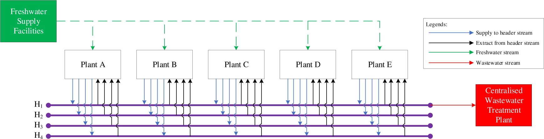
The concentration range of each header is controlled by the operator of the CWRH system ‒ the CWRH accept only water sources with controlled concentrations of the other contaminant within boundaries. Figure 1 shows the illustration of an industrial site with four one-way CWRH system.
The aim of the work is to study the impact of multiple CWRH on both consumer’s operating cost and operator’s payback period.
Industrial site with four one-way CWRH system
Detailed methodology of TS-CWI has been discussed by Fadzil et al. [21]. The methodology of TS-CWI is revised and listed below:
Step 1: Data of water sources and water demands (Flowrate and contaminant concentration) for each Plant (i) involved in the system is extracted;
Step 2: Specify the number of Headers (j) and concentration range for each Header (j);
Step 3: Flowrate, mass load and concentration of water source from Header (j) received by Plant (i) is calculated using eq. (1-3):
(1)
(2)
(3)
where F [t/h] is flowrate, m [kg/h] is mass load, C [ppm] is contaminant concentration, i is the plant number and j is the number of headers.
Step 4: Total Site Centralised ‒ Water Cascade Table (TSC-WCT) [23] is constructed to calculate the minimum Plant (i) water source extracted from Header (j). Freshwater requirement and wastewater generated for Plant (i) are also obtained in Step 4. The value can be obtained in column 3 of the final TSC-WCT. Concentration is the same as the concentration of water source received. The mass load is calculated using eq. (4):
(4)
TSC-WCT is calculated based on two key steps below:
Step 4(i): Header flowrate [FH((j)] targeting. Header flowrate is targeted from the lowest quality to the highest quality. Freshwater flowrate (FFW) is then targeted as the highest quality of water sources available;
Step 4(ii): Header flowrate [FH((j)] adjustment. Header flowrate is then adjusted from the highest quality to the lowest quality;
Step 5: Flowrate of plant (i) unutilised water source is calculated using eq. (5):
(5)
Step 3 to 5 is repeated for the subsequent Plant (i) until the last plant along CWRH. TS minimum freshwater requirement (FTS,FW) is calculated using eq. (6). The TS wastewater flowrate (FTS,WW) sent to the centralised Wastewater Treatment Plant (WWTP) is calculated using eq. (7). The mass load (mTS,WW) and concentration (CTS,WW) of TS wastewater are calculated using eq. (8) and eq. (9):
(6)
(7)
(8)
(9)
The remaining unutilised water source from each header are sent for treatment to the centralised WWTP. Water sources with contaminant concentrations exceed header concentration range set in Step 2 are also sent to the centralised WWTP. It is suggested for the operator to only bought sufficient water sources to satisfy the water demand of the system.
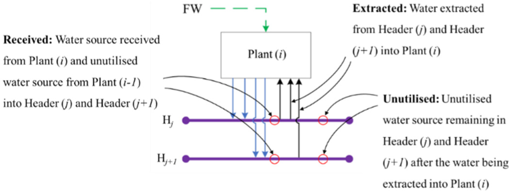
Figure 2 shows the location of received, extracted and unutilised flowrate in TS-CWI.
Location of received, extracted and unutilised flowrate in TS-CWI
An industrial site that consists of five plants located along the CWRH is solved to illustrate the methodology. Single pseudo-contaminant (TDS) is assumed for the water network. The TS initial freshwater requirement is 2,865 t/h, and the initial wastewater generation is 2,635 t/h. The analysis is performed on the Case Study, with one CWRH to up to four CWRH to study the effects of increasing the number of CWRH. Data of water sources and demands of each plant is obtained from Fadzil et al. [21] presented in Table 1.
Water sources and demands data
| Plant A | Plant B | Plant C | Plant D | Plant E | ||||||||||
|---|---|---|---|---|---|---|---|---|---|---|---|---|---|---|
| Stream name | F [t/h] | C [ppm] | Stream name | F [t/h] | C [ppm] | Stream name | F [t/h] | C [ppm] | Stream name | F [t/h] | C [ppm] | Stream name | F [t/h] | C [ppm] |
| S-A1 | 200 | 50 | S-B1 | 50 | 50 | S-C1 | 100 | 70 | S-D1 | 20 | 100 | S-E1 | 20 | 50 |
| S-A2 | 80 | 80 | S-B2 | 250 | 110 | S-C2 | 120 | 260 | S-D2 | 80 | 125 | S-E2 | 100 | 80 |
| S-A3 | 80 | 100 | S-B3 | 150 | 130 | S-C3 | 85 | 260 | S-D3 | 100 | 200 | S-E3 | 40 | 130 |
| S-A4 | 140 | 150 | S-B4 | 150 | 250 | S-C4 | 200 | 350 | S-D4 | 100 | 250 | S-E4 | 25 | 350 |
| S-A5 | 200 | 220 | S-B5 | 70 | 300 | S-C5 | 200 | 400 | S-D5 | 50 | 800 | S-E5 | 25 | 400 |
| D-A1 | 200 | 0 | D-B1 | 50 | 20 | D-C1 | 100 | 0 | D-D1 | 20 | 0 | D-E1 | 20 | 0 |
| D-A2 | 80 | 50 | D-B2 | 250 | 50 | D-C2 | 120 | 100 | D-D2 | 80 | 50 | D-E2 | 100 | 50 |
| D-A3 | 80 | 50 | D-B3 | 150 | 100 | D-C3 | 85 | 125 | D-D3 | 100 | 100 | D-E3 | 40 | 80 |
| D-A4 | 140 | 100 | D-B4 | 150 | 200 | D-C4 | 200 | 500 | D-D4 | 100 | 150 | D-E4 | 25 | 100 |
| D-A5 | 200 | 120 | D-B5 | 300 | 250 | D-C5 | 200 | 500 | D-D5 | 50 | 300 | D-E5 | 25 | 100 |
Note: F is flowrate, C is concentration, Source is denoted as S in-stream name and Demand is denoted as D in-stream name
The minimum and maximum concentrations of water sources accepted by the CWRH is kept constant at 10 to 400 ppm. The interval is increased by 20 ppm to find the optimum CWRH concentration range for each Case Studies. The optimum header concentration range is obtained at the highest consumer’s total saving and lowest operator’s payback period. Water sources with contaminant concentrations above 400 ppm are not accepted by the system for water reuse but sent directly to the centralised WWTP.
Determining the optimum CWRH concentration range is vital since it can affect the economics of the system. The optimum concentration range for each CWRH is determine based on consumer and operator perspectives.
As a consumer, the CWRH concentration range is optimum if the system capable of providing the most significant cost reduction for each plant involved in the system.
As an operator, the CWRH concentration range is optimum if the system is profitable and return in a short amount of time. Table 2 shows the comparison of optimum CWRH concentration range between consumer and operator perspectives for each Case Studies.
From Table 2, additional CWRH have a positive effect on freshwater reduction whether the system is built from the consumer or operator perspectives as multiple CWRH gives more flexibility for consumer to choose a wide range of water source to be efficiently reused for their processes. The consumer might opt a water source at lower tariff to reduce their operating cost.
From the consumer perspectives, additional CWRH increase the total cost savings by 19.2% and increase the operator’s payback period by 0.4 years. Case Study 3H and 4H benefit consumer the most with 73.0 and 78.4% of total cost saving. Conversely, the operator suffered a negative profit for both systems. It is not ideal for the operator to build three or four CWRH system. The operator could have just built a single CWRH and attain a payback at 4.1 years.
From the operator perspectives, the operator can obtain the lowest payback of 3.5 years by constructing a two CWRH system. Adding the second CWRH gives a 0.6 years faster payback period with further total savings of 50.9% for the consumer.
Comparison of optimum CWRH concentration range between consumer and operator perspectives
| Case Studies | Operator perspectives | Consumer perspectives | |||||||
|---|---|---|---|---|---|---|---|---|---|
| 1H | 2H | 3H | 4H | 1H | 2H | 3H | 4H | ||
| CWRH concentration range [ppm] | H1 | 10-400 | 10-80 | 10-80 | 10-80 | 10-400 | 10-140 | 10-140 | 10-140 |
| H2 | 80-400 | 80-320 | 80-240 | 140-400 | 140-160 | 140-160 | |||
| H3 | 320-400 | 240-280 | 160-400 | 160-220 | |||||
| H4 | 280-400 | 220-400 | |||||||
| Consumer | Freshwater reduction [%] | 61.9 | 76.8 | 77.2 | 77.2 | 61.9 | 82.0 | 82.5 | 86.3 |
| Wastewater reduction [%] | 89.6 | 89.6 | 89.6 | 89.6 | 89.6 | 89.6 | 89.6 | 89.6 | |
| Total cost savings [%] | 48.8 | 50.9 | 52.6 | 53.4 | 48.8 | 68.0 | 73.0 | 78.4 | |
| Operator | Total capital cost [USD] | 3,189,229 | 2,912,607 | 3,475,252 | 4,004,524 | 3,189,229 | 3,843,766 | 4,976,003 | 5,384,442 |
| Total operating cost [USD/year] | 4,017,375 | 2,815,500 | 3,622,270 | 4,371,209 | 4,017,375 | 4,838,051 | 7,159,606 | 7,711,508 | |
| Profit earned [USD/year] | 9,270,294 | 19,065,309 | 17,215,525 | 15,781,768 | 9,270,294 | 7,071,590 | −2,020,347 | −1,146,793 | |
| Payback period [years] | 4.1 | 3.5 | 3.7 | 3.9 | 4.1 | 4.5 | - | - | |
| NPV at 23 years [USD] | 58,470,790 | 116,475,872 | 104,279,666 | 94,726,865 | 58,470,790 | 40,223,488 | −18,079,980 | −13,048.566 | |
It is crucial for the operator to determine the optimum CWRH concentration range since incorrect CWRH concentration range could upturn the payback period by manifold. Using Case Study 2H as an example, the payback period can be reduced up to 1 year if the first CWRH concentration range is 10-140 ppm instead of 10-80 ppm. Proper identification of the optimum concentration for each CWRH of Case Study 3H and 4H could ensure a profitable business for the operator.
In conclusion, if the optimum CWRH concentration range is determined from the consumer’s perspective (to obtain the highest total cost-saving), the operator could suffer negative profit as in Case Study 3H and 4H (see Table 2). Conversely, if the optimum CWRH concentration range is determined from the operator perspective (to obtain the lowest payback period), the system is certain to yield a profit to the operator with the lowest payback period achievable in any Case Study (see Table 2). In either situation, the consumer still gains benefits no less than 48.8% because the system provides reuse opportunity for each consumer to reduce dependency solely on freshwater. Therefore, the optimum CWRH concentration must be determined from the operator perspectives (lowest payback period).
The practicability of the system is evaluated through economic analysis. Both perspectives of consumer and operator are applied to compare between each Case Studies. Capital and operating cost of piping, pump and WWTP are calculated based on Seider [24]. The calculations basis as indicated:
Operating hours are 8,000 h/year;
The construction period is 3 years, plant life is 20 years and depreciation is 10% of the total capital cost;
Consumer buying cost per unit [USD/t] for freshwater, H1, H2, H3 and H4 are 3, 2.8, 2.6, 2.4 and 2.2;
Consumer selling cost per unit [USD/t] for H1, H2, H3 and H4 are 1.4, 1.3, 1.2 and 1.1;
One unit of the pump is used per pipeline. The material (FM = 1.35) is cast steel and the type (FT = 1.50) is single-stage pump (1,800 shaft rpm);
Cost per unit of electricity is USD 0.1/kWh;
Cost per unit of WWTP operation is USD 0.5/t;
Cost per unit of pipeline construction is USD 100/m;
Distance between processes within Plant (i) is 0.1 km, and the distance between Plant (i) and Plant (i+ 1) is 1 km. The total distance from Plant A to E is 4 km. Adding an additional 1 km from Plant E to the centralised WWTP;
Cost of piping and pumping is incurred by a plant that received water source from other plants [only for Case Study based on Superstructure Optimisation (SO)].
The system is purely built and incurred by the operator of the system. Hence, the consumer only needs to consider the cost of operating their plant. This includes the cost of freshwater, buying header water sources from the system and cost of wastewater treatment.
Initially, without any efforts of integration, each plant depends wholly on freshwater to satisfy its water demand and directly send their unused wastewater for treatment. The initial TS cost of freshwater is USD 68,760,000, while the TS cost of wastewater treatment is USD 10,540,000. The initial TS annual operating cost is USD 79,300,000.
Consumer are able to minimise their dependency on freshwater as the CWRH system provide lower purity water sources to maximise water reuse among plants at an industrial site. Table 3 and Table 4 shows the consumer economic analysis summary.
Consumer economic analysis summary (in terms of flowrate)
| Case Study | Freshwater | Wastewater | ||||
|---|---|---|---|---|---|---|
| Initial [t/h] | Minimum [t/h] | Reduction [%] | Initial [t/h] | Minimum [t/h] | Reduction [%] | |
| 1H | 2,865 | 1,091.6 | 61.9 | 2,635 | 275 | 89.6 |
| 2H | 2,865 | 666 | 76.8 | 2,635 | 275 | 89.6 |
| 3H | 2,865 | 652.7 | 77.2 | 2,635 | 275 | 89.6 |
| 4H | 2,865 | 653.5 | 77.2 | 2,635 | 275 | 89.6 |
| SO | 2,865 | 608.5 | 78.8 | 2,635 | 378.4 | 85.6 |
Consumer economic analysis summary (in terms of cost)
| Case Study | Initial [USD/year] | Final [USD/year] | Final operating cost [USD/year] | Overall savings [%] | ||||
|---|---|---|---|---|---|---|---|---|
| Freshwater | Wastewater | Freshwater | H buy | H sell | Wastewater | |||
| 1H | 68,760,000 | 10,540,000 | 26,199,432 | 39,719,668 | 26,432,000 | 1,100,000 | 40,587,100 | 48.8 |
| 2H | 68,760,000 | 10,540,000 | 15,984,359 | 47,360,809 | 25,480,000 | 1,100,000 | 38,965,168 | 50.9 |
| 3H | 68,760,000 | 10,540,000 | 15,665,833 | 45,477,795 | 24,640,000 | 1,100,000 | 37,603,628 | 52.6 |
| 4H | 68,760,000 | 10,540,000 | 15,682,962 | 44,032,977 | 23,880,000 | 1,100,000 | 36,935,938 | 53.4 |
| SO | 68,760,000 | 10,540,000 | 14,604,545 | - | - | 1,513,778 | 16,118,323 | 79.7 |
Note: H buy indicate consumer buy water source from the CWRH, H sell indicate consumer sell their water source to the CWRH
Wide range of water sources available enables the consumer to be efficiently reused for their processes. For example, process D-D5 required water sources at 300 ppm. In Case Study 1H, the available water sources are S-DH1 at 202.3 ppm, while in Case Study 4H, the available water sources are S-DH4 at 252.6 ppm. Water sources from H4 are at a lower tariff compared to H1 and still can be used by process D-D5. Which, in turn, reducing the operating cost. Therefore, an increase in the number of CWRH has a benefit of freshwater reduction.
In terms of wastewater reduction, there are no changes in Case Studies with CWRH system because the maximum concentrations of water sources accepted by the system is fixed at 400 ppm for all Case Studies.
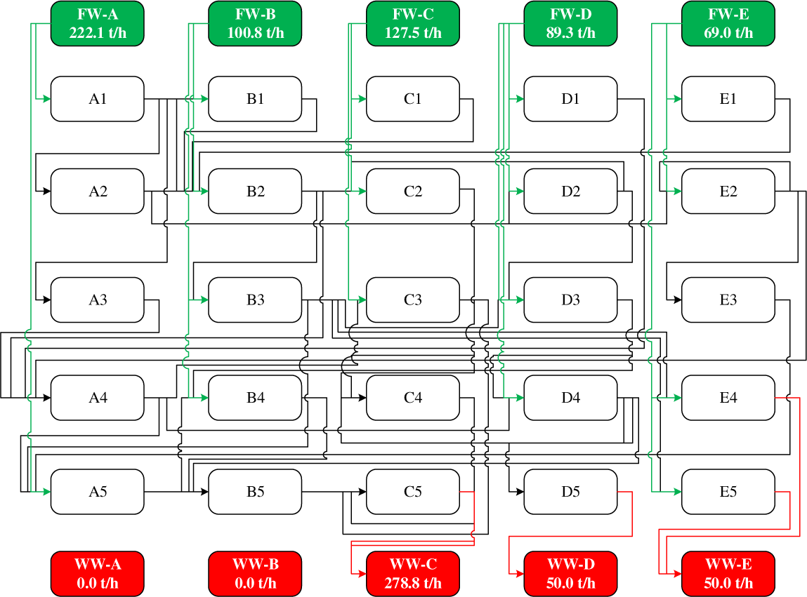
Water Integration via SO is the direct integration of water source and demands from each plant. The integration is conducted by assuming all water sources and demands from different plants as one plant. The method is preferable to achieve higher overall reduction (79.7%) on both freshwater and wastewater. This is because the cost of buying and selling of water source from CWRH is not applicable. However, regardless of having a higher reduction in freshwater and wastewater, the resulted water network is too complicated to be implemented. The piping arrangement may become more costly if the cost factor of distance is added. The issues of industries sharing information and confidential data for plant integration may make it less practical. The capital cost and operating cost of each industry may increase since they are required to build their own WWTP. On the other hand, the Case Study could have been improved by implementing CWRH system as the integration method to promote water reuse between each plant. The system is more practical to be applied in real-life situation since the water network is more straightforward and less costly as compared to the SO method. CWRH system is operated by a third-party. This ensures that confidential data of each plant is protected. The operator is also the investor for the centralised WWTP in the industrial site area. The optimal TS water network via SO is illustrated in Figure 3.
Optimal TS water network via superstructure optimisation
As the operator, both operating and capital cost of the system are included in the economic analysis. Capital cost includes the cost of pump, piping and centralised WWTP. The operating cost includes the electricity cost of pumping, the operation of WWTP and the buying of water sources from industries. The profit comes from the sales of water sources to industries. The operator economic analysis summary is presented in Table 5.
Operator economic analysis summary
| Case Study | Capital cost [USD] | Operating cost [USD/year] | Sales [USD/year] | Payback period [year] | ||||
|---|---|---|---|---|---|---|---|---|
| Piping | Pump | WWTP | Pump | WWTP | H buy | H sell | ||
| 1H | 600,000 | 17,007 | 2,572,221 | 570,173 | 3,447,202 | 26,432,000 | 39,719,668 | 4.1 |
| 2H | 1,200,000 | 24,188 | 1,688,419 | 1,029,844 | 1,785,657 | 25,480,000 | 47,360,809 | 3.5 |
| 3H | 1,710,000 | 32,844 | 1,732,408 | 1,763,392 | 1,858,878 | 24,640,000 | 45,477,795 | 3.7 |
| 4H | 2,230,000 | 40,416 | 1,734,107 | 2,509,481 | 1,861,728 | 23,880,000 | 44,032,977 | 3.9 |
Note: H buy indicate operator buy water source from the consumer, H sell indicate operator sell their water source to the consumer
Capital cost increase as the number of CWRH increases because more CWRH requires more piping and pumping. Cost of buying water sources from industries is high for 1H because all quality of water sources hinge on only one water tariff. Increasing the number of CWRH can reduce the cost where the operator can buy the lower quality of water sources at a lower tariff.
Sales for Case Study 1H is the lowest because industries have a limit on only the quality of water sources other than freshwater. This also reflects on the cost of WWTP, where water sources are poorly utilised, and a high amount of water sources is sent to the centralised WWTP for treatment.
With four units of CWRH, the consumer can buy water sources at four different tariffs. This reduces the sales for the operator because some of the industries might choose to procure water source at lower tariff to reduce their own operating cost.
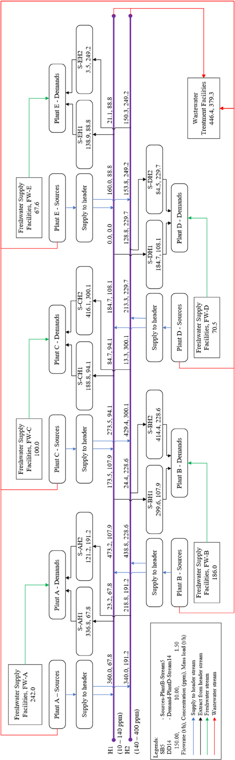
Two units of CWRH gives the lowest payback period for the operator with only 3.5 years. The total capital cost of the system is USD 2,912,607 comprises a total of 12 km pipeline with pumps and the centralised WWTP. The total annual operating cost of the system is USD 2,815,500 comprises of pumping electricity cost (USD 1,029,844), WWTP operation (USD 1,785,657) and procurement of water sources from each plant (USD 25,480,000). Total profits earned from selling water sources are USD 47,360,809. The optimal TS water network with two units of CWRH is shown in Figure 4.
Optimal TS water network with two units of CWRH
As a final point, determining the optimal CWRH concentration range has to be carefully considered in order to avoid any drawbacks to the operator. The optimum CWRH concentration range needs to be determined from the operator perspective to ensure that the system is profitable and that the lowest payback period is achieved for the system. Determining CWRH concentration range from the consumer perspective may result in a negative profit for the operator. In addition, increasing the number of CWRH does have a trade-off effect on both consumer’s total cost savings and operator’s payback period. The consumer can reduce their operating cost with a higher number of CWRH because it enables the industry to purchase lower quality water at a lower tariff. However, increasing the number of CWRH reduces the operator’s sales because a higher number of CWRH provide more ranges of water sources with a lower tariff. The consumer could opt to only procure lower tariff, thereby reducing the operator profit. A higher number of CWRH also increases the cost to build the system.
Taking everything into account, 50.9% of consumer’s operating cost can be reduced with two units of CWRH. This also yields the most benefits to the operator of the system with the lowest payback period of 3.5 years. Three or four units of CWRH could have given higher total cost savings for the consumer (52.6 and 53.4%), at the expense of a longer payback period for the system (3.7 and 3.9 years).
Future research and development work will consider multiple contaminants in the system. The addition of the regeneration unit also needs to be studied to further improve the CWRH system. Heat recovery, fouling factor, and detail analysis of the pipeline size is essential for future improvement of the system.
This work financial support aided by Fundamental Research Grant (FRGS) from the Ministry of Education Malaysia under Vote R.J130000.7809.4F918 and Universiti Teknologi Malaysia (UTM) Research University Grant (GUP) under Vote Q.J130000.2509.19H34 and Q.J130000.3509.05G96. Additional financial support is provided by the EC-funded project Sustainable Process Integration Laboratory (SPIL), funded as project No. CZ.02.1.01/0.0/0.0/15_003/0000456, by Czech Republic Operational Programme Research and Development, Education, Priority 1: Strengthening capacity for quality research under the collaboration agreement with the UTM, Johor Bahru, Malaysia. The authors are appreciatively acknowledged.
- , The United Nations World Water Development Report 2015, Water for a Sustainable World, United Nations Educational, Scientific and Cultural Organization (UNESCO), 2015
- , The United Nations World Water Development Report 2017, Wastewater: The Untapped Resources, United Nations Educational, Scientific and Cultural Organization (UNESCO), 2017
- ,
Wastewater Minimisation ,Chemical Engineering Science , Vol. 49 (7),pp 981-1006 , 1994, https://doi.org/https://doi.org/10.1016/0009-2509(94)80006-5 - ,
Series: De Gruyter Textbook, De Gruyter ,Process Integration and Intensification: Saving Energy, Water and Resources (2nd extended ed.) , 2018 - ,
Dealing with Plant Geography and Piping Constraints in Water Network Design ,Process Safety and Environmental Protection , Vol. 74 (4),pp 273-276 , 1996, https://doi.org/https://doi.org/10.1205/095758296528626 - ,
Material Reuse Modeling: A Case Study of Water Reuse in an Industrial Park ,Journal of Industrial Ecology , Vol. 2 (4),pp 79-92 , 1998, https://doi.org/https://doi.org/10.1162/jiec.1998.2.4.79 - ,
New Structure and Design Methodology for Water Networks ,Industrial and Engineering Chemistry Research , Vol. 40 (26),pp 6140-6146 , 2001, https://doi.org/https://doi.org/10.1021/ie000835i - ,
Design Methodology for Flexible Multiple Plant Water Networks ,Industrial and Engineering Chemistry Research , Vol. 46 (14),pp 4954-4963 , 2007, https://doi.org/https://doi.org/10.1021/ie061299i - ,
Synthesis of Direct and Indirect Interplant Water Network ,Industrial and Engineering Chemistry Research , Vol. 47 (23),pp 9485-9496 , 2008, https://doi.org/https://doi.org/10.1021/ie800072r - ,
Targeting the Minimum Water Flow Rate using Water Cascade Analysis Technique ,AIChE Journal , Vol. 50 (12),pp 3169-3183 , 2004, https://doi.org/https://doi.org/10.1002/aic.10235 - ,
Flowrate Targeting for Threshold Problems and Plant-Wide Integration for Water Network Synthesis ,Journal of Environmental Management , Vol. 88 (2),pp 253274 , 2008, https://doi.org/https://doi.org/10.1016/j.jenvman.2007.02.007 - ,
Segregated Targeting for Multiple Resource Networks using Decomposition Algorithm ,AIChE Journal , Vol. 56 (5),pp 1235-1248 , 2010, https://doi.org/https://doi.org/10.1002/aic.12050 - ,
Design of Inter-Plant Water Network with Central and Decentralized Water Mains ,Computers and Chemical Engineering , Vol. 34 (9),pp 1522-1531 , 2010, https://doi.org/https://doi.org/10.1016/j.compchemeng.2010.02.024 - ,
Mathematically Rigorous Algebraic and Graphical Techniques for Targeting Minimum Resource Requirement and Interplant Flow Rate for Total Site Involving Two Plants ,Industrial and Engineering Chemistry Research , Vol. 51 (8),pp 3401-3417 , 2012, https://doi.org/https://doi.org/10.1021/ie202135w - ,
Industrial Water Management by Multiobjective Optimization: From Individual to Collective Solution Through Eco-Industrial Parks Design of Water Network ,Journal of Cleaner Production , Vol. 22 (1),pp 85-97 , 2012, https://doi.org/https://doi.org/10.1016/j.jclepro.2011.09.011 - ,
Optimal Interplant Water Networks for Industrial Zones: Addressing Interconnectivity Options Through Pipeline Merging ,AIChE Journal , Vol. 60 (8),pp 2853-2874 , 2014, https://doi.org/https://doi.org/10.1002/aic.14516 - ,
Inter-plant Water Integration with Considerations of Water Supply Constraint and Differential Water Price ,Chemical Engineering Transactions , Vol. 45 ,pp 139-144 , 2015, https://doi.org/https://doi.org/10.3303/CET1545024 - ,
Synthesis of Industrial Park Water Reuse Networks Considering Treatment Systems and Merged Connectivity Options ,Computers and Chemical Engineering , Vol. 91 ,pp 289-306 , 2016, https://doi.org/https://doi.org/10.1016/j.compchemeng.2016.02.003 - ,
Synthesis of Water Networks for Industrial Parks Considering Inter-Plant Allocation ,Computers and Chemical Engineering , Vol. 91 ,pp 307-317 , 2016, https://doi.org/https://doi.org/10.1016/j.compchemeng.2016.03.013 - ,
Accounting for Central and Distributed Zero Liquid Discharge Options in Interplant Water Network Design ,Journal of Cleaner Production , Vol. 171 ,pp 644-661 , 2017, https://doi.org/https://doi.org/10.1016/j.jclepro.2017.09.236 - ,
Industrial Site Water Minimisation via One-Way Centralised Water Reuse Header ,Journal of Cleaner Production , Vol. 200 ,pp 174-187 , 2018, https://doi.org/https://doi.org/10.1016/j.jclepro.2018.07.193 - ,
Up-to-date Tools for Water-System Optimization ,Chemical Engineering Magazine , Vol. 111 (1),pp 30-41 , 2004 - ,
Water Cascade Analysis for Single and Multiple Impure Fresh Water Feed ,Chemical Engineering Research and Design , Vol. 85 (8),pp 1169-1177 , 2007, https://doi.org/https://doi.org/10.1205/cherd06061 - ,
, Product and Process Design Principles: Synthesis, Analysis and Evaluation (3rd ed.) , 2010