


In the last decades, there has been an increasing demand for quantitative methods for sustainability assessment. This led, in particular, to the proliferation of composite indexes, that can provide a numerical synthesis of multiple assessments from different perspectives. The United Nations Environment Programme (UNEP) developed the Sustainability Assessment of Technologies Methodology (SAT) [1] to provide a general framework for structuring and supporting the assessment process in the context of sustainable development. The SAT methodology can be applied to a variety of situations, and with complexity ranging from policy making at the government (strategic) level to comparing technology options at the local community (operational) level. The European Commission created the Competence Centre on Composite Indicators and Scoreboards (COIN) [2] whose mission is to provide and continuosly improve reliable tools for building robust composite indexes. A relevant area of application for sustainability assessment is offered by cities, often, in this context, a composite index is designed to focus on a specific aspect. For example, the Sustainable Cities Index (SCI) by Arcadis [3] explores city sustainability from the perspective of the citizens, trying to assess how a city meets their needs. This also leads to a classification of the cities into four clusters, based on their similarity to eight “archetypes”. SCI is currently applied to 100 cities from all over the world, and is based on three pillars (“People”, “Planet” and “Profit”) evaluated on 13, 11 and 7 indicators, respectively. Another example is provided by the Clean Air Scoreboard (CAS) by Clean Air Asia Initiative [4], that focuses on the city’s management of air pollutants. CAS has been applied in 19 Asian cities from nine countries, and integrates three aspects, related to actual air pollution levels, potential to face the problem, and existing policies/actions. A sample of some most relevant city sustainability indexes are described and compared in Kilkiş [5]. It is worth noting that the assessment of cities is not limited to sustainability issues. For example, the European Digital City Index (EDCi) [6] shows how cities support digital entrepreneurship. A detailed discussion of EDCi, and a comparison to other indexes with similar aims, can be found in Bannerjee et al. [7].
In recent years, a growing interest has been attracted by a specific city-centred composite index, namely the Sustainable Development of Energy, Water and Environment Systems (SDEWES) Index. At the time of writing, this index is applied to an integrated sample of 120 cities, results, partially aggregated data and related explicatory material are maintained in [8]. This index was designed to address the integrated development of energy, water and environment systems (EWE systems for short) including societal and technological aspects, and with a particular focus on the goal of decoupling energy and resource usage from carbon dioxide (CO2) emissions. It is based on the following seven main dimensions:
Energy usage and climate;
Penetration of energy and CO2 saving measures;
Renewable energy potential and utilization;
Water usage and environmental quality;
CO2 emissions and industrial profile;
Urban planning and social welfare;
R&D, innovation and sustainability policy.
Each dimension is evaluated based on five indicators some of which, in turn, are obtained by aggregating sub-indicators. Technical details on the computation of the SDEWES Index are provided later in this work. It is worth noting that some dimensions (1, 4-6) essentially provide a picture of the current status of a city EWE system, while others (2, 3, 7) evaluate the existing actions and the city potential to improve sustainability. Moreover, dimensions 1 and 5 are more directly related to the main focus of the SDEWES Index, since they measure the quality of the urban systems in terms of efficiency and CO2 emissions, respectively, accordingly, these two dimensions are assigned a greater relevance (i.e., a larger weight) in the computation of the index. The SDEWES Index was originally applied to a sample of 12 South East Europe (SEE) cities [9]. A sample of 22 Mediterranean port cities were considered in Kılkış [10], where an “Energy Scenario Tool” was proposed to evaluate (in terms of the index values and ranking) the impact of possible actions improving the EWE system of a city. A further set of 25 world cities were considered in Kılkış [11], where a “Benchmarking Tool” is devised to compare the performance of cities. Moreover, the “city pairing” process is introduced as a tool for supporting policy learning and best practices exchange. This process consists in finding pairs of cities with similar behaviour (either under or below average) on all dimensions. Results of city pairing are reported also in Kılkış [12], where a further sample of 18 SEE cities is considered. In Kılkış [13], a further sample of 26 world cities is evaluated, and a “normative scenario” (see discussion below) for Rio de Janeiro is analysed. The data for another sample of 18 world cities are compiled in Kılkış [14]. An in-depth discussion of the results (including, but not limited to, sensitivity and scenario analysis, and city pairing) for the overall integrated sample of 120 cities addressed so far can be found in Kilkiş [5], an overview is given in Kilkiş [15]. In particular, the areas of best practice characterizing the top ten cities in the SDEWES Index ranking are pointed out in Kilkiş [5]. The analysis reveals that all these cities show best practices in the areas of urban energy systems and/or of CO2 emissions. This seems to suggest that energy/emission decoupling is a key factor for attaining a high level of sustainability. Some remarks along this line of thought are provided later in this work.
An in-depth analysis of the SDEWES Index goes beyond the scope of this work. Nevertheless, it is important to point out a few relevant aspects here. First, the computation of the SDEWES Index involves a substantial amount of work for data collection. To begin with, a city to be evaluated via the SDEWES Index must have a Sustainable Energy Action Plan (SEAP) and maintain reliable statistics on its local energy system. Furthermore, collected data usually require pre-processing, e.g. for computing main indicators based on sub-indicators. These issues are skipped in this work, where the analysis starts after data collection and pre-processing. Second, the SDEWES Index is descriptive in nature but it also has a relevant prescriptive value. Indeed, it may help city planners to find successful policies for enhancing the sustainability of local energy systems. This can be obtained in several ways, the most obvious ones being spreading awareness and identifying best practices. In this direction, a methodologically more involved approach is provided by the city pairing process cited above. Beyond policy learning, the goal should be to adopt the SDEWES Index as the objective function to optimize when selecting or designing policies, in order to take integrated actions addressing several aspects of sustainability [5], [15]. Last but not least, the SDEWES Index can be used to track the evolution of local EWE systems, and this means, in particular, that it allows to evaluate the impact of sustainability policies. This aspect is clearly pointed out in Kılkış [13], in relation with some medium-long term commitments (with target spanning between 2035 and 2060) undertaken by the City of Rio de Janeiro. The impact of these commitments on the SDEWES Index is evaluated, which allows to forecast the evolution of the index value for Rio in the next decades. It can be argued that, during this period, a comparison of actual and envisioned results may provide useful feedback on the policy implementation status. That is, the SDEWES Index has the capability not only to evaluate the envisioned impact of sustainability policies, but also to assess, and keep track of, their actual implementation. However, in order to fully exploit this “evaluate and assess” capability, the index should be computed consistently throughout a possibly wide time horizon. This is one of the issues addressed by the present work.
By definition, a composite index is a numerical aggregation of measures arising from different indicators. These measures are expressed in many different scales, ranging from purely qualitative or ordinal (that essentially sort elements into categories) to strongly cardinal ones, that have a sound physical meaning and specific units (such as “dollars” or “tons of CO2”). The aggregation of multiple evaluations on different scales is the subject of Multiple Criteria Decision Analysis (MCDA) [16]. In fact, any composite index can be seen as the numerical solution of an underlying MCDA problem, in particular, for the “ranking problematic” (see e.g. Greco et al. [16]), i.e. establish a complete order among a set of alternatives. A description (including a detailed visual representation) of the MCDA problem underlying the SDEWES Index can be found in Carli et al. [17], where the ranking obtained by the SDEWES Index is compared to the one of a hybrid method (merging AHP [16] with SDEWES Index computation at the indicator level) for a sample of four cities. Since long time, and far beyond the link to composite indexes, MCDA methods have been applied in the field of sustainable development. The survey in Thies et al. [18] mentions 142 articles that apply MCDA and related methods to support or replace standard sustainability assessment methods. Another recent survey [19] lists 94 articles (dating 1995-2017) where MCDA assessment methods include social aspects in the evaluation of infrastructure sustainability. In a bibliography of more than 2,000 articles on PROMETHEE-GAIA applications [20] over 40% of the entries deal with energy, environment or water management. A survey devoted to ELECTRE methods [21] shows that 153 papers (out of the 544 application papers addressed there) deal with natural resources and environmental management. The role of MCDA for sustainability assessment has been investigated also from a theoretical point of view. The features of several MCDA methods, and their suitability for sustainability assessment, are discussed in Cinelli et al. [22], while Greco et al. [16] provides a critical analysis, in light of MCDA theory, of common practices and implicit assumptions in composite indicators for sustainability.
In short, this work deals with composite indexes from an MCDA point of view. More precisely, some concepts and tools developed in the context of MCDA are applied to the ranking problem underlying a composite index. Two main topics are addressed: the “rank reversal” effect, and the application of visual support tools. It must be remarked that these topics may be of concern in a broad context, virtually for any index or benchmarking technique, not limited to sustainability issues. However, no efforts towards generality are made in this work, on the contrary, the above topics are addressed only in the context of the SDEWES Index. This implies that some observations and results are motivated by, and related to, the features and aims of the SDEWES Index, however, it must be kept in mind that here the SDEWES Index is adopted essentially as a paradigmatic example. The motivations for this choice should be clear in light of the above discussion, and include the availability of data, the wide scientific literature on the subject and, last but not least, the promising potential of the SDEWES Index as a decision supporting tool. In particular, the analyses conducted in the present work were made possible by the availability of the underlying data both at the dimension level [8] and (almost completely) at the indicator level [9]-[14]. For other indexes, data are not always made available, e.g., the Sustainable Cities Index [3] only provides the final scores and a graphical representation of normalized data.
In MCDA terminology, a rank reversal occurs if the order of preference between two alternatives changes when an alternative is added to or removed from the decision problem. This means that the relative ranking of a pair of alternatives depends on the whole set of alternatives, and not only on the pair itself, in fact, an MCDA method exposed to rank reversal lacks of the so called “independence” property. Rank reversal, or equivalently “non-independence”, is known to affect many MCDA methods, and has been the subject of a long-lasting debate, see for example [23], [24] and the references therein. In the context of MCDA methods for sustainability assessment rank reversal is specifically addressed in Cinelli et al. [22]. In practice, the occurrence of rank reversals is likely to be rather limited, and can be considered a minor problem in light of the aim and scope of the SDEWES Index. On the other hand, since the index is designed to address an inherently evolving reality, non-independence implies that the results may not be computed consistently throughout a wide time interval. This can be limiting if the goal is to adopt the index as a tool for evaluating and assessing policies, to this aim, it would be useful to devise a “stable” (i.e., “independent”, or “rank-reversal free”) version of the SDEWES Index. Here it will be shown that the MCDA theory offers a viable approach to obtain such version. It turns out that devising a stable index, although demanding in terms of technological expertise, is relatively easy from a mathematical point of view.
A plethora of data visualization techniques are available today, and they are widely used in support of sustainability assessment analyses. As for the SDEWES Index, just to mention a couple of examples: radar (or spider-web) charts are used in the SDEWES Index Benchmarking Tool [11], while geographical maps and stacked charts are combined in the “SDEWES City Index Atlas” [8], [15]. In addition, special techniques have been developed, e.g. the three-dimensional visualization proposed for the City Sustainability Index [25]. Visualization tools have been widely studied also in the context of MCDA, to address the “description problematic” [16], see Miettinen [26] for an overview. A well-known example is the Graphical Analysis for Interactive Aid (GAIA) methodology, that has been developed as a visual companion to PROMETHEE methods [16]. GAIA includes several graphic and interactive tools, in particular the “GAIA plane”, based on the projective approach originally proposed in Mareschal and Brans [27]. The GAIA plane allows to reveal interesting relations between criteria and/or alternatives of an MCDA problem. Other tools similar to the GAIA plane have been proposed, e.g., the “Co-plot” method: see Raveh [28] for a description and a comparison to the GAIA plane. It is worth noting that Co-plot exploits more sophisticated statistical data analysis techniques compared to GAIA, on the other hand, Co-plot is not linked to a specific MCDA method, as GAIA is. In the present work, the GAIA plane is adapted to work with dimensions and indicators of the SDEWES Index. The benefits of this approach are shown, and some drawbacks are pointed out. Consequently, a new and simple visual tool is proposed. This tool shows explicitly and exactly some information that is somehow hidden or approximated in the GAIA plane. Some particular features of the new tool are exploited, first to provide a graphical representation of the scenario analyses discussed in Kilkiş [5] and Kilkiş [13], and then to point out some aspects related to the decoupling of energy use from CO2 emissions.
The layout of this paper is as follows. In Section 2 rank reversal is discussed, together with a possible approach for obtaining a stable index. Section 3 provides the definitions of the visual tools and points out their main features, while Section 4 shows the application of the tools to the SDEWES Index, in particular to data aggregated at the dimension level. The last section contains a few conclusions and suggestions for further work.
In MCDA terms, dimensions and indicators of the SDEWES Index define a two-level criteria hierarchy. The top level consists of seven macro-criteria, corresponding to dimensions D1, D2, …, D7. At the bottom level appear the actual criteria, i.e., the main indicators. There are exactly five indicators (criteria) for each dimension (macro-criterion) and this gives an MCDA problem with m = 35 criteria. The alternatives correspond to cities, and their number n varies depending on the sample. The current version of the index [8] considers a sample of n = 120 cities, that integrates the samples reported on in detail in the literature [9]-[14]. For each x>[1], [7] and y>[1], [5] denote by Ex,y(Cj) the evaluation of city Cj according to the yth criterion of dimension Dx. The computation of the SDEWES Index involves four steps:
Statistical treatment of outliers by means of winsorization;
Normalization of evaluations within each indicator;
Computation of a sub-index for each dimension;
Aggregation of sub-indexes.
As described in [5], [13] outliers are identified and treated by means of higher order moments, namely skewness and kurtosis. A single step of winsorization consists in replacing all the occurrences of the highest evaluation value by the second-highest one, this step is iterated until skewness and kurtosis fall below 2 and 3.5, respectively, or until a maximum of 5% of the values have been modified. A complete list of the indicators that required winsorization for the current 120-city sample is provided in Kılkış [14]. In the normalization step the evaluations are mapped onto the interval [0, 10], for maximization criteria, the normalized value is defined as:
(1)
while for minimization criteria the equation is:
(2)
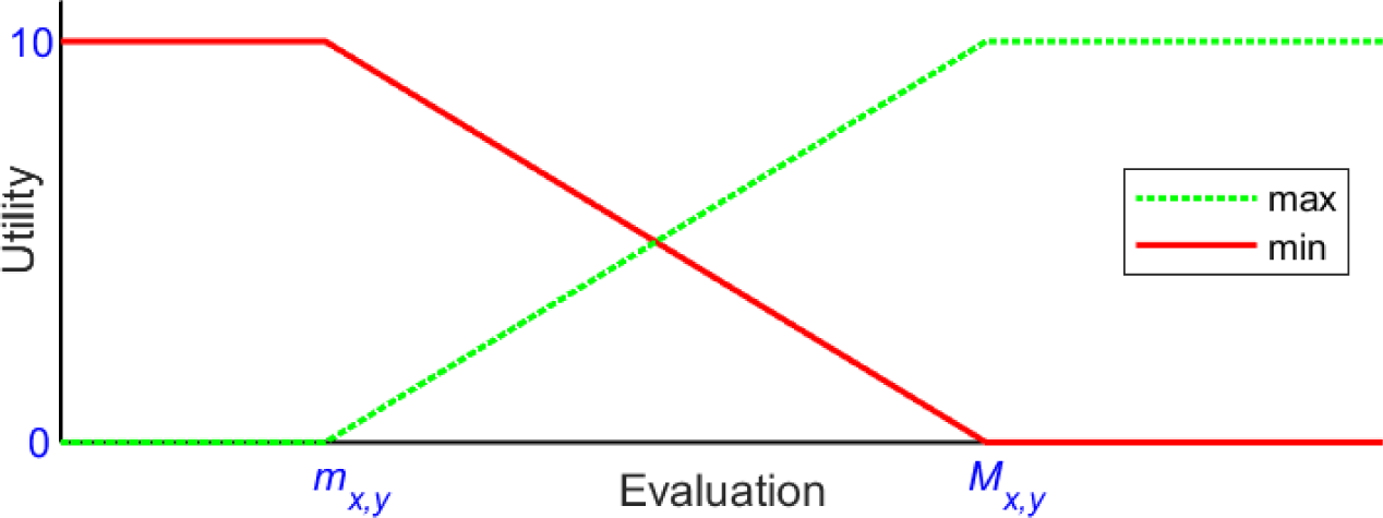
where mx,y and Mx,y denote the minimum and the maximum values Ex,y(Cj) across all cities, after winsorization. Note that for each indicator the best (respectively, worst) value is mapped into the normalized value 10 (respectively, 0). For each dimension an aggregated sub-index falling in the interval [0, 50] is defined as:
(3)
Finally, the SDEWES Index is obtained as:
(4)
where ax = 0.225 for x = 1 and x = 5, and ax = 0.11 for the other dimensions. Note that the weights α sum to one, thus the index is normalized in [0, 50]. It is worth noting that in the earlier works [9]-[11] the factor 10 was not included in eq. (1) and eq. (2), thus the index and each sub-index where normalized in [0, 5]. Furthermore, the treatment of outliers by winsorization was omitted.
The SDEWES Index can be seen as the result of the well-known “weighted sum” MCDA method, see e.g. Pomerol and Barba-Romero [29] for a discussion. Weighted sum assigns to each alternative a score defined as a weighted sum of its normalized evaluations, this can be seen in eq. (4), where each normalized indicator of dimension Dx is given the weight ax. The weighted sum is a totally compensatory method, where the weaknesses of an alternative can be compensated by its strengths. This means that the SDEWES Index of a city can be good even if some of the indicators have a quite poor evaluation. Technically, a score SI(Cj) does not depend on the dispersion of the values Ix,y(Cj) and/or Ax(Cj), i.e., on these values being rather similar across the whole set of indicators and/or dimensions, or spread in a large interval. On the contrary, other MCDA methods are sensitive to dispersion: this is the case e.g. of TOPSIS, as pointed out in Yoon [30]. Note that the visual tool proposed later has the ability to capture, at least partially, the information related to dispersion.
The weighted sum method is known to be exposed to rank reversal, due to its normalization phase. An expository example is shown in Wang and Luo [23], note the normalization technique in that example is the same as in eq. (1) and eq. (2), except that the factor 10 is missing. It follows that also the SDEWES Index is potentially exposed to rank reversal, indeed, it is easy to see that the normalization process violates the independence property, since the results of eq. (1) and eq. (2) depend on mx,y and Mx,y, and thus on the whole city sample. Clearly, the bounds for an indicator can change with time, as long as new cities are added to the sample, or due to changes in the city evaluations. It is interesting to point out what happens to the normalized values Ix,y(Cj) when either mx,y or Mx,y changes. It can be shown (technical details are rather straightforward and omitted here) that improving the best evaluation (respectively, worsening the worst evaluation) makes the Ix,y(Cj) decrease (respectively, increase).
This can be considered as a reasonable and fair reaction to the setting of a higher or a lower standard, due to the arrival of a new very good or very poor city. Note that the use of winsorization may prevent these changes to take place, or at least filter off the ones with the most consistent impact. On the other hand, a straightforward application of the winsorization process to wider and wider samples may lead to unexpected effects, as shown by the following example.
Consider indicator 4 of dimension 3, “Renewable energy in electricity production”, measured as a percentage. For the set of 58 cities obtained from the samples in [9]-[11] kurtosis is above the maximum threshold 3.5, as a consequence, the best value 100 (city of Tirana) is replaced by the second-best value 80 (city of Bogotá), thus M3,4 = 80 and the normalized value is ten for both cities. Consider now the whole current sample of 120 cities: in this case, kurtosis is below the threshold and no winsorization is needed, thus M3,4 = 100 and (since m3,4 = 1) Bogotá receives a value approximately 8, while Tirana retains the value 10. Note that 5 of the cities from [12]-[14] have an evaluation greater than 80, and this may (at least partially) justify the fall of the score for Bogotá. However, the same result (i.e., no winsorization needed) is obtained if the evaluations of these 5 cities are replaced by values smaller than 80. The conclusion is that the score of a city in an indicator can drop due to the insertion of cities whose evaluation is worse than the one of that city.
It must be remarked that the behaviour pointed out in Example 1 did not affect the computation of the indicator, since winsorization was not applied in [9]-[11], moreover, data seem to suggest that no outliers are likely to be detected if the current 120-city sample is further extended. Nevertheless, Example 1 suggests that despite of (and may be due to) winsorization the bounds mx,y and Mx,y may change rather unpredictably in the long run. This means the score of a city may be artificially increased or decreased, regardless of the actual evolution of its local EWE system. In short, the index is not stable. Note that from an MCDA point of view the lack of stability cannot be considered as a methodological flaw, since it is a consequence of the lack of independence, which is almost ubiquitous in MCDA methods. The question is whether this stability issue is relevant in practice. Two objections can be raised:
Objection 1. EWE systems are inherently dynamic entities: technological development, as well as social pressure, lead to setting higher and higher standards, to which a city should continuously struggle for complying, see e.g. [5]. Accordingly, a local system should be evaluated in relation to other evolving systems, rather than based solely on its own features;
Objection 2. The SDEWES Index is a yet evolving tool. Comparing the definitions in [5], [13]-[15] to the ones in [9]-[12] it turns out that some indicators have been evaluated on different scales, replaced, or merged together, while new ones have been added. It can also be argued that the SDEWES Index should retain its dynamic nature, in order to comply with the evolution of technology and the improvement of EWE systems.
In light of these objections, one should accept the idea that the SDEWES Index returns a sequence of snapshots, each one relative to the current city sample and corresponding performances, and to the current set of indicators. After all, this does not seem to seriously affect its descriptive power, and has a quite limited impact on its prescriptive value. On the other hand, the lack of stability may be drawback when the SDEWES Index is considered as a tool for evaluating and assessing the impact of sustainable development policies. Indeed, this task requires to compute the index in a consistent way both in the evaluation phase and throughout the (possibly long) time horizon set by the policy target. Note that in this case instability is not only due to larger city samples, but also (and may be above all) to the evolution of local EWE systems. Therefore, in order to fully exploit the evaluating and assessing capabilities of the SDEWES Index, it seems necessary to tackle the stability issue explicitly. Ideally, the goal should be to obtain a version of the index that can at the same time:
On one side, evaluate and track the evolution of EWE systems consistently and independently of each other;
On the other side, allow the comparison and benchmarking of an expanding set of cities.
In the rest of the section this goal is pursued exploiting some principles and tools from MCDA theory. Clearly, a stable version of the SDEWES Index implies a stable set of indicators and sub-indicators, including their scale of measure, in what follows, this is assumed to be the case. A further premise is necessary, and is based on the following observation. The sample in Kılkış [11] changed the bounds of mx,y and/or Mx,y for 20 out of the 35 indicators, w.r.t. previous samples [9], [10], on the contrary, also due to winsorization, the sample in Kılkış [12] turned out to fall within previous bounds. However, this does not necessarily mean that the index is evolving towards stability due to the addition of new samples. As suggested by Example 1 (and actually confirmed by Objection 1) a significant shift of the bounds may be expected in the future for some of the indicators. On the other hand, for other indicators the bounds for the 120-city sample are already sufficiently stable, or at least provide a reliable picture of the situation, including possible future trends.
Observe that the combination of winsorization and normalization implicitly define for each criterion a (normalized and piecewise linear) utility function Fx,y(v) mapping each evaluation Ex,y(Cj) onto the interval [0, 10]. For a maximization criterion, this function assigns full utility to evaluations above the threshold Mx,y, and null utility to evaluations below the threshold mx,y, evaluations in [mx,y, Mx,y] are linearly mapped onto [0, 10]. For a minimization criterion, the role of the thresholds is symmetric, as shown in Figure 1. Note that utility functions are defined on the whole domain of possible criterion evaluations, that (at least in principle) may be unbounded, even if in most cases (e.g., for a percentage) upper and lower bounds are readily available. Therefore, the flat zones on the left and on the right appear whenever the interval [mx,y, Mx,y] does not cover the domain, clearly, if winsorization detects outliers, they end up falling below these flat zones. It can be observed that the utility function (for maximization) resembles the “Linear” preference function of PROMETHEE [16], [31]. In particular, mx,y and Mx,y play the role of the “indifference” and “preference” thresholds Q and P, respectively. Although in different contexts, these function share the common approach of mapping high and low values onto the extremes of the normalization interval.
Based on the above utility functions, the SDEWES Index may be interpreted in terms of Multiple Attribute Utility Theory (MAUT: see e.g. [16], [29]) as an additive utility model:
(5)
Utility function for maximization and minimization criteria
where each utility function Fx,y is given the weight fx,y = ax. Such additive model, once defined, can be later applied to any sample of cities, and applied again to the same city whenever some of its evaluations have changed. Remark that the score computed by eq. (5) does no longer depend on the city sample, since each city is evaluated independently, thus the additive model satisfies the independence property, i.e. is not exposed to rank reversal. As observed explicitly in Cinelli et al. [22], MAUT (not necessarily restricted to additive models) is the only MCDA approach that provides completely rank reversal free solutions. Clearly, in order to define the additive model in eq. (5) the utility functions Fx,y(v) must be defined once and for all. This amounts to say that a stable version of the SDEWES Index is obtained if the current bounds mx,y and Mx,y are fixed as definitive, possibly after some suitable adjustments. Unfortunately, as discussed earlier, this operation is in general not safe: for some indicators, current bounds may not be representative of future trends. In these cases, reasonable bounds should be found, and this may be a challenging task for those indicators (in particular, maximization ones) for which evaluations are expected to improve substantially in the future. Note that the task can be simplified in light of a few preliminary observations, including (but not limited to) the following:
Some indicators (e.g. those for dimension D2, but also I5,5, I6,2, I7,1, I7,2) are measured on essentially qualitative scales, that are specifically defined to aggregate the results of sub-indicators, and for which it should be easy to derive reasonable bounds;
For some indicators measured in percentage (e.g. I3,4, I3,5, I4,2, I7,5), mx,y and/or Mx,y are equal or very close to 0 and 100, respectively;
for some indicators (e.g. I1,1, I1,2, I1,4, I4,5, I5,1, I5,2, I7,4), Mx,y is two or three orders of magnitude larger than mx,y: in these cases, it should be safe to shift mx,y to zero,
For most maximization (minimization) indicators it seems suitable to set the current mx,y(Mx,y) as a minimum performance thresholds under (over) which a null utility must be assigned.
Moreover, an additive model is not restricted to use the utility functions Fx,y(v) described above. These functions are not monotonically increasing or decreasing, since they show flat zones where evaluations are not distinguished from each other. Thus it may be appealing to consider smoothed version of these functions. A smooth utility function does not require to set the bounds mx,y and Mx,y, and may provide a more sophisticated model including e.g. saturation effects. A suggestion for a smooth function is again offered by PROMETHEE, in particular by the “Gaussian” preference function, a version rescaled within [0, 10] will be considered here:
(6)
In addition, a “cubic” version of G(v) will be used:
(7)
Both functions G(v) and H(v) are monotonically increasing, with shape changing from convex to concave, and such that G(d) = H(d), as shown in Figure 2. The following example gives a hint of how these smooth functions may be used for one particular indicator.
Piecewise linear and smooth utility functions
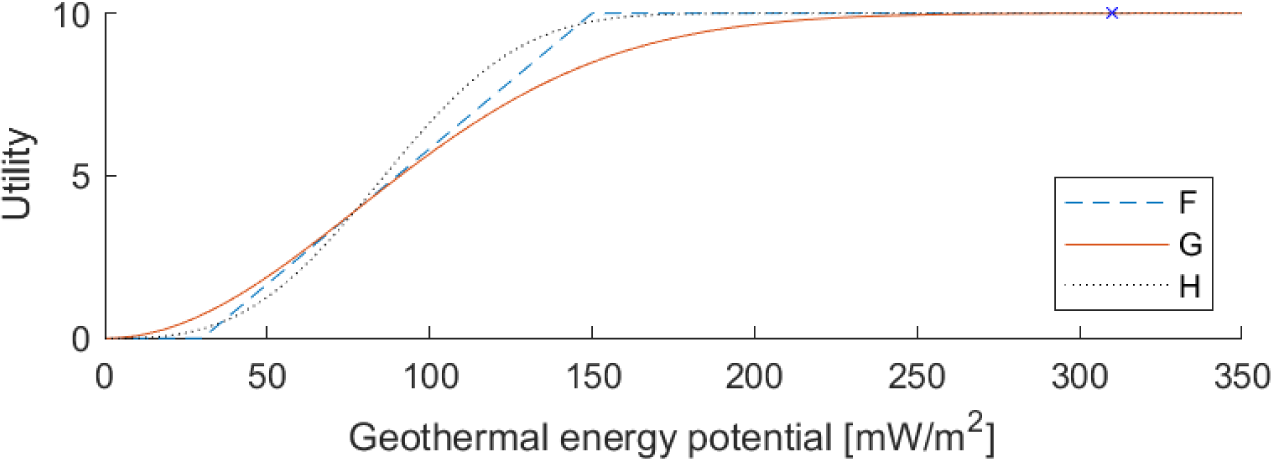
Consider indicator 3 of dimension D3: “Geothermal energy potential” [mW/m2] for which the current bounds (after winsorization) are m3,3 = 30 and M3,3 = 150 with a single outlier, namely Reykjavík, with an evaluation of 310 as shown in Figure 2 [11], [14]. Assume that possible evaluations outside the bounds are taken into consideration, and handled according to the following principles:
Positive values below m3,3 should be assigned a non-zero utility;
For values over M3,3 the utility function should be increasing, but with a rather fast saturation effect.
This can be obtained exploiting the functions G(v) or H(v). In order to obtain three curves F3.3(v), G3.3(v) and H3.3(v) close to each other the parameter d is set so that F3.3(d) = G3.3(d) = H3.3(d).
Note that G3.3(mx,y) ≅ 0.727 and G3.3(Mx,y) ≅ 8.485: the current bounds are not mapped onto extreme utility values, since some utility values must be reserved for evaluations over M3,3 and below m3,3. Using G(v) instead of F(v) the score for Reykjavík remains almost unchanged [G3.3(310) ≅ 9.997 instead of F3.3(310) = 10] while the scores for the other cities are shrunk within an interval of length G3.3(Mx,y) - G3.3(mx,y) ≅ 7.758. That is, the outlier is distinguished from the other cities (according to the above principles) but the discriminating power among these cities is reduced. If the shrinking deriving from G3.3(v) is considered excessive, then a function with a sharper behaviour may be used instead, for example, H3.3(v) gives an interval of wider length H3.3(Mx,y) - H3.3(mx,y) ≅ 9.455.
It must be remarked that the principles inspiring the utility function in Example 2 are purely explicative, and do not necessarily match with the actual aim of the indicator. Moreover, the functions G(v) and H(v) have been chosen solely for the sake of simplicity, while the method for choosing the parameter d is rather straightforward, if not naïve. Clearly, much more involved mathematical tools can be exploited to find suitable utility functions. If necessary, further degrees of flexibility may be obtained, e.g. considering different normalization intervals and/or different weights for some indicators. This allows to concentrate efforts on technical issues, such as derive a clear picture of the current level of development, foresee a reasonable trend of evolution on a medium-long term, and (last but not least) evaluate the utility that should be associated with future improvements in relation with the aims and scope of the index. The conclusion that can be drawn from the above discussion is that choosing suitable utility functions may be challenging but is definitely possible. In other words, the SDEWES Index is a promising candidate for the process of moving from weighted sum to an additive utility model, which in light of MCDA theory is the unique approach leading to stability, i.e. to satisfy the independence property.
As mentioned above, several kinds of visual tools have been devised in the context of MCDA. Here, the interest is concentrated on tools representing the overall structure of the decision problem, in particular on the GAIA plane. Similar tools have been proposed in the literature, such as the aforementioned CoPlot method, but GAIA is apparently the simplest and the most widely known. Here, the GAIA plane is adapted for the SDEWES Index, addressing both the top level and the bottom level of the criteria hierarchy. Furthermore, a new tool will be presented, namely the “Index/Dispersion plane”. From a visual point of view, the new tool is very close to the GAIA plane, and conveys comparable information. Similarities and differences between the two methods will be discussed, and illustrated by means of some examples. On the computational side, the Index/Dispersion plane bears some resemblance with the CoPlot method since, in both cases, the alternative representation is found first, and the criteria representation is derived from it. There are, however, strong differences between the two approaches. In the tool proposed here, both city and criteria representations are found in a very simple way, and have a clear interpretation in terms of the underlying MCDA problem. On the contrary, CoPlot finds the mapping of the alternatives exploiting rather sophisticated statistical methods for multi-dimensional scaling, and finds the representation of each criterion solving (heuristically) a rather difficult non-linear optimization problem. Furthermore, CoPlot representations have no interpretation in terms of the underlying problem, while the Index/Dispersion plane conveys explicit information related to the SDEWES Index.
In the GAIA plane, alternatives, criteria and weights are jointly represented by points on a plane. More precisely, each criterion is graphically represented by a “vector”, i.e. a segment from the origin to the corresponding point, the vector representing the weights is usually referred to as the “stick”. The primary plane is identified by the axes U (horizontal) and V (vertical), a third axis W allows to define the secondary planes (U, W) and (V, W). This representation is obviously approximated, since it only shows the projections on a plane of points in a space of dimension p, i.e. the number of criteria. The method also provides a measure of the quality of the representation, which can be seen as the percentage of information retained after projection. The GAIA plane allows to visualize several aspects of an MCDA problem, such as conflicting criteria or sensitivity to changes in the weights, see Mareschal and Brans [27] and Greco et al. [16] for a detailed discussion. The interesting features for the present work can be summarized as follows:
Alternatives with similar characteristics appear close to each other in the plane;
Criteria expressing similar (respectively: opposite, uncorrelated) preferences are represented by vectors oriented in approximatively similar (respectively: opposite, orthogonal) directions;
Points corresponding to better alternatives for a criterion are likely to be found moving in the direction of the corresponding criterion vector, similarly, the stick shows the direction where globally better alternatives can be found;
The length of a vector denotes the reliability of the visual information it conveys: a short length suggests a high loss of information due to projection.
In order to find the axes U, V and W, GAIA applies Principal Component Analysis (PCA) to the matrix of profiles computed by the PROMETHEE method. The profile of an alternative is a (row) vector of scores, one for each criterion. Profiles are particularly suitable for PCA since they are normalized in [-1, 1] and centered, i.e. the sum of scores over all alternatives is zero for each criterion. Obviously, in the context of the SDEWES Index profiles do not exist, but PCA can be applied to available data that are normalized, even if not centered. There are two possibilities here, namely, apply PCA at the top level or at the bottom level of the criteria hierarchy. In the former case, a city Cj is represented by the sub-indexes Ax(Cj), for x = 1, 2, …, 7, recall that the sub-indexes are normalized in [0, 50]. In the latter case, PCA is applied separately for each dimension Dx, and a city Cj is represented by its scores Ix,y(Cj), y = 1, 2, …, 5, normalized in [0, 10]. From now on, the generic term “criterion” is used to denote either a dimension (at top level) or an indicator (at bottom level). In both cases, let M denote the n × p “score matrix”, where n is the number of cities and p is either 7 or 5, each city Cj is represented by row j of M. The PCA method for finding the axes U, V, W and the qualities of the projection planes can be summarized as follows:
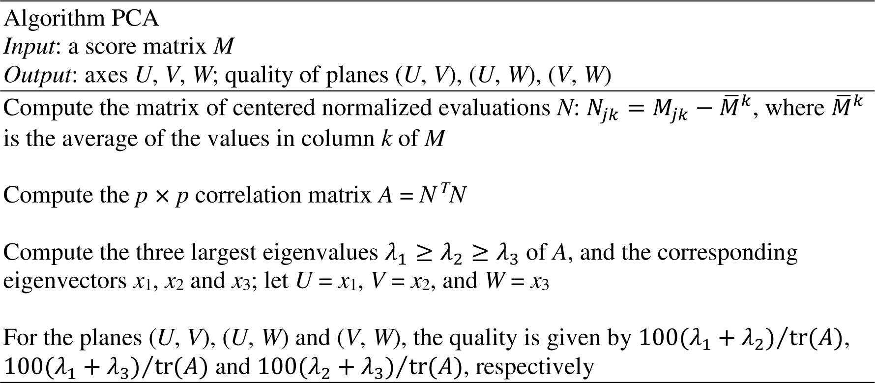
Given the axes, the coordinates of relevant points on the plane (U, V) can be computed as shown below, the computation for the secondary planes (U, W) and (V, W) is similar:
City Cj has coordinates (Nj.U, Nj.V), where Nj. is row j of N;
Criterion k has coordinates (Uk, Vk);
The stick has coordinates (wTU, wTV).
Note that the weights are represented by a unit-length vector w, where w = α/||α||2 at top level, while at bottom level w = u/||u||2, where u = [1, 1, 1, 1]T. Recall that the weight vector is not considered in the PCA algorithm. Consequently, the aggregated score (the SDEWES Index at top level, a sub-index at bottom level) is not represented exactly on the GAIA plane. The stick shows a direction of expected growth, but this information may be quite approximated, in particular if the stick length is short. This is one of the motivations that lead to the proposal of a different visual representation.
As discussed earlier, the weighted sum method is totally compensatory, i.e. it is not sensitive to dispersion of criteria values. Accordingly, the SDEWES Index does not take dispersion into consideration. On the other hand, distribution patterns of sub-indexes are relevant for city pairing [5], [12], [15], thus a measure of dispersion may be helpful in that context. The GAIA plane reveals some information about dispersion, since the direction orthogonal to the stick is somehow related to dispersion, however, this information is not explicit, and in some cases can be quite approximated. The tool proposed here aims at visualizing an aggregated score (horizontal coordinate) and the corresponding dispersion (vertical coordinate) explicitly and exactly. Also in this case, the method can be applied at two levels: at top level, the aggregated score is the SDEWES Index, while at bottom level it is the sub-index Ax(Cj) for a given dimension x, in both cases, the input data are contained in the n × p score matrix M, as defined for the GAIA plane.
Clearly, many different measures of dispersion can be adopted: a straightforward geometrical approach is followed here. Consider first the top level, where each city Cj is represented by the sub-indexes Ax(Cj), contained in row j of the score matrix M. Thus city Cj is a point in the space of dimension p = 7, and weights are represented by the unit length vector w = α/||α||2. For each city Cj let , where πj = Mj.w. Note that πj is the length of the projection of onto the axis defined by w, while the vector dj is orthogonal to this axis, thus ||dj||2 is the Euclidean distance of from the axis. It can be easily checked that:
(8)
Therefore, to obtain homogeneous scales, the normalized distance:
(9)
is chosen as a measure of the dispersion of the sub-indexes representing city Cj. The extension to the bottom level is immediate: in this case, for dimension x, city Cj is represented by indicators , is a point in the space of dimension p = 5, and the vector u = [1, 1, 1, 1, 1]T replaces the vector α, i.e. w = u/||u||2. The value πj and the vector dj are defined as for the top level, and it turns out that:
(10)
Therefore, similar to eq. (9), dispersion is measured by .
Based on the representation of cities, a two-dimensional visualization of the criteria can be defined. The idea is that criterion k is represented by the point of coordinates , where and are a measure of the correlation of the criterion with the aggregated score and the dispersion, respectively. In particular, the Pearson correlation coefficient will be used, recall that this coefficient is normalized in [-1, 1]. Both at top and bottom level, criterion k corresponds to column k of the score matrix M, while aggregated score and dispersion can be represented by the n-dimensional vectors π and δ defined above. Thus the horizontal coordinate of criterion k is defined as:
(11)
where is the average of column k of M, while π ̅ is the average value of vector π. The vertical coordinate is defined as in eq. (11), replacing π by δ. Graphically, criterion k is represented by a vector from the origin to the point . Remark that (differently from GAIA) each of the two coordinates conveys sound information on the underlying MCDA problem. The horizontal coordinate shows whether, and up to what extent, the aggregated preferences agree with the ones expressed by the criterion. The vertical coordinate shows whether a good performance on the criterion comes at the expenses of a larger dispersion among criteria. An interesting feature of the Index/Dispersion approach is that criteria coordinates can be computed considering only a subset of the n cities. This allows, in particular, to partition the overall sample into sub-samples (e.g., quartiles) and obtain distinct representations of criteria separately for each sub-sample. These representations can be compared to each other, in order to spot those cases where the relations between criteria differ depending on the sub-sample. Note that a similar process is not possible with the GAIA plane, where the representation of criteria is determined univocally by the axis U and V, and cannot be related to sub-samples. It is worth mentioning that data analysis separated by quartiles has been exploited in [5], [12], [13], [15], see e.g. figure 4 in Kilkiş [5], where graphical representations are given both at the index and at the sub-index level.
Similar to the GAIA plane, a joint representation of cities and criteria is also possible. To this aim, the criteria representation should be translated so that its origin moves to the coordinates given by the average aggregated score and the average dispersion. Equivalently, the city coordinates should be replaced by their centered counterparts, i.e. by differences w.r.t. averages. Moreover, a rescaling is necessary, since and are normalized within [-1, 1], while city coordinates are numbers in [0, 50]. The joint representation allows to visualize the relations between criteria and cities, i.e. better cities for criterion k are likely to be found in the direction defined by the corresponding vector . In other words, a criterion communicates a “visual ranking” of the cities, which is expected to be similar to the actual ranking defined by the criterion. Technically, the visual ranking is defined by the “visual scores” of the cities: for criterion k, and for city Cj, the visual score is the length of the projection of (the point representing) Cj on the axis representing k, or equivalently, by the scalar product between and the coordinates of Cj. At top level, according to eq. (8) and eq. (9), the visual score of Cj for dimension Dk is given by:
(12)
At bottom level, according to eq. (10), the visual score of Cj for indicator k of dimension Dx is given by:
(13)
Exploiting eq. (12) and eq. (13) it is possible to give a measure of the reliability of the visual ranking offered by criterion k. This can be done by computing the Pearson correlation coefficient between the actual scores, defined by column k of the input score matrix M, and the visual scores defined by Pk. Note that a similar measure of reliability can be given for the GAIA plane as well. In the plane (U, V), and similar for secondary planes, the visual score of Cj for criterion k is given by:
(14)
As shown later, this allows to compare the reliability of the visual rankings provided by GAIA and by Index/Dispersion.
In the Index/Dispersion representation cities are processed independently of each other. Therefore, a change in the city sample or in the data representing a city cannot affect the representation of another city. This may be referred to as a sort of independence property of the proposed approach. Note that independence does not extend to criteria, since their representation is based on global information, i.e., on scores and dispersion of all the cities in the sample. Suppose now that the method is applied, in conjunction with a stable version of the SDEWES Index, for a sufficiently long period of time, during which the EWE systems of many cities are likely to evolve significantly. Accordingly, the Index/Dispersion representation of a city will change over time depending on the city’s system evolution, but independently of other cities. In other words, each city will define a “trajectory” on the Index/Dispersion plane, and trajectories will be independent of each other. Looking at things the other way round, a city trajectory may be defined in advance by the envisioned results of a particular policy: in this case, that trajectory defines a stable representation of the expected results throughout the whole time horizon of the policy. This may be useful to support the process of evaluating and assessing the impact of sustainability policies. The conclusion is that the proposed approach is quite appealing as a visual companion of a stabilized SDEWES Index. Remark that the GAIA plane does not show a similar level of reliability. The PCA method is inherently unstable, since the projection axes depend on the underlying score matrix M. When new cities are added, or when some evaluations change, the projection planes are modified, and this affects the whole picture returned by the GAIA plane.
This section reports some examples of the plots that can be obtained with the adapted GAIA plane and with the Index/Dispersion method. The goal is to point out similarities and differences between the two approaches, trying to shed light on their strengths and weaknesses. To this aim, the figures will come in pairs (except for the last one) which allows to compare the visual representations provided by the two methods for the same set of information. It must be remarked that the examples shown here are not intended to provide an extensive analysis of the (substantial amount of) information conveyed by the SDEWES Index, thus they are not expected to reveal, unless incidentally, any peculiar or unexpected feature. The ultimate goal is to demonstrate the soundness and suitability of the visual tools. For reasons of space, and for uniformity of presentation, only top level is addressed, bottom level provides a larger set of data representations, but does not reveal any new feature of the proposed tools. Unless stated otherwise, all the figures refer to the current 120-city sample available from [8]. Figures obtained from GAIA are limited to the (U, V) plane, and are somehow simplified w.r.t. the usual appearance, omitting axes and bounding boxes, similar, rulers are often omitted in the Index/Dispersion plots. Nevertheless, all the relevant information is given within each figure. In some cases, specific subsets of cities will be individuated by means of different markers and/or by tracing the convex hull of the corresponding set of points in the plane.
The first pair of figures illustrates the main difference between the two approaches, namely, the capability of representing exactly the value of the SDEWES Index. To this aim, the four quartiles individuated by the index values are represented. Figure 3 shows the GAIA plane with the stick showing the approximate direction of increase for the SDEWES Index. Observe that the length of the stick is 0.912, that is sufficiently close to one, this means that the unit length vector w = α/||α||2 is quite close to its projection on the (U, V) plane. However, some information is lost in the projection process, as can be expected from the quality value. Indeed, quartiles appear in the right order along the stick direction, but with overlapping convex hulls. Obviously, no overlapping appears in the Index/Dispersion representation of Figure 4, that allows to point out two interesting details:
For cities in the bottom quartile (91-120) both the SDEWES Index and the dispersion are spread in a much wider interval compared to the middle quartiles, up to a minor extent, the same holds true for the top quartile too;
Within the top quartile, the best index values are found in the top-right corner, i.e. show a relatively high dispersion, in other words, and excellent overall performance can be obtained even with relatively wide differences between single dimension performances.
GAIA: city quartiles and stick

Index/Dispersion: city quartiles and simulation trajectories
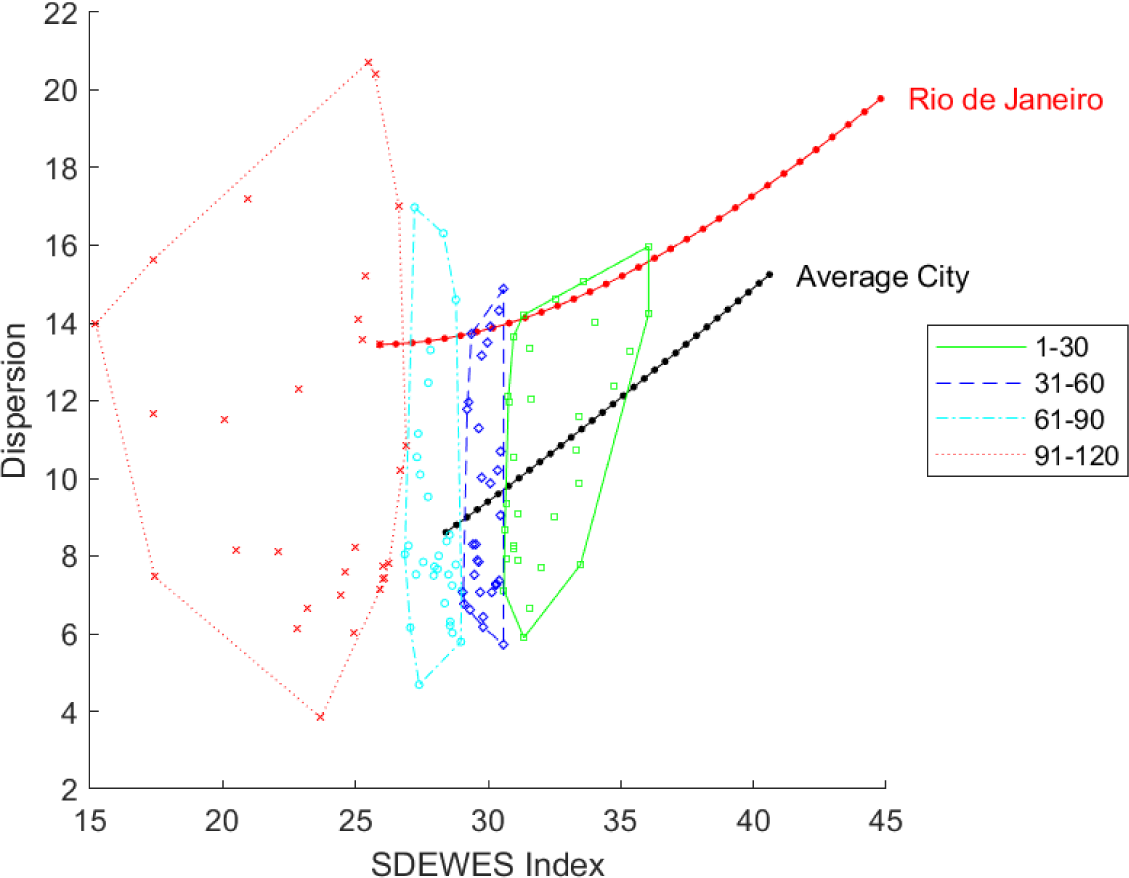
Figure 4 also shows two trajectories individuated by simulating the evolution of a city along time. The simulation for Rio de Janeiro is based on the results for the normative scenario addressed in Kılkış [13]. The simulation for the “Average City” is taken from a scenario addressed in [5], [15], where a fictitious city evolves, in each dimension, from the average to the maximum of the corresponding sub-index values in the current 120-city sample. In both cases, the simulation assumes a transition from the current situation (year 2019) to the situation foreseen for the target year 2050. Here, for simplicity, the transition is assumed to be linear in time, markers show the expected situation for each year in the time horizon. Even if the transition is linear, the trajectory is not necessarily linear, since the measure of dispersion is not linear. It can be observed that the proposed scenarios lead to a substantial increase not only for the SDEWES Index (as expected) but also for dispersion.
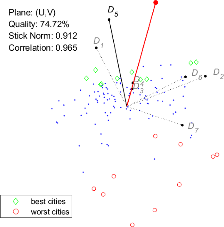
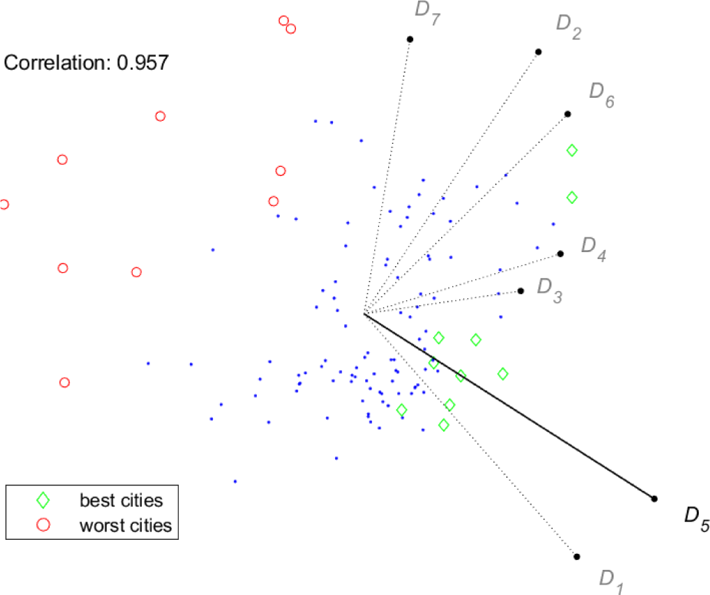
The goal of the next figures is to show that the two tools have the same capability of representing the relations among criteria and the relations between criteria and cities. Moreover, the information they convey have similar reliability. To this aim, conjoint plots of criteria and cities are provided, and further visual information is added as follows. In each plot, a specific dimension Dx is selected, and the best ten and the worst ten cities for Dx are highlighted. This gives a visual intuition of the quality of the visual ranking of the cities. Moreover, the measure of reliability defined above, here denoted by “Correlation”, is provided for each plot. In Figure 5 and Figure 6, the selected dimension is D5. For both tools, the correlation value is very close to one, and indeed, the visual ranking of the cities seems quite close to the actual one, with best and worst cities appearing on opposite sides of the city cloud. Note that for both tools the length of the vector representing D5 is high.
GAIA: conjoint plot, best/worst cities for D5
Index/Dispersion: conjoint plot, best/worst cities for D5
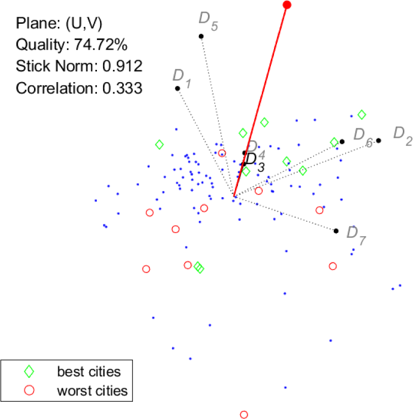
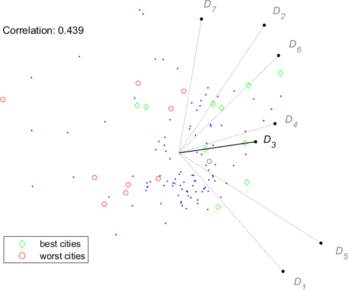
In Figure 7 and Figure 8, the selected dimension is D3. In this case, the correlation value is rather low, and indeed the visual ranking appears much less reliable, with some of the best and worst cities mixing together around the origin. Note that both the length of the vector representing D3 and the correlation value are higher for Index/Dispersion than for GAIA. The relatively poor visual performance of dimension D3 can be related to its low correlation to the index, and this behaviour seems to suggest that some cities do not yet fully exploit their renewable energy potential in their energy supply systems, in this area, a remarkable example of best practice is given by the city of Reykjavík (the diamond close to the point defining D3 in Figure 8) that decarbonized its power sector [5], [14].
GAIA: conjoint plot, best/worst cities for D3
Index/Dispersion: conjoint plot, best/worst cities for D3
Besides the above observations on the visual ranking of cities, Figures 5-8 show that the two tools provide remarkably similar representations of the criteria. The only evident difference is the length of the vectors representing dimensions D3 and D4. Keeping in mind the meaning of the stick for GAIA, it is possible to draw some conclusions supported by both tools:
Up to different extents, the first six dimensions bring some similarity to the overall index, with D5 showing the strongest correlation ;
On the contrary, dimension D7 is almost uncorrelated to the index, this seems to suggest that an innovative city is not necessarily a sustainable city;
There is a partial conflict (or better a lack of correlation) between two sets of dimensions, namely, D1 and D5 opposed to D2, D6 and D7, in particular, this is revealed by dispersion, or equivalently by the direction orthogonal to the stick on the GAIA plane.
As for the last observation, it is not easy to find a simple interpretation. A possible explanation may be as follows. On one side, dimensions D2, D6 and D7 are somehow related to the degree of social-cultural development of a city (in terms of sustainability awareness, welfare, education, innovation, etc.) and thus can be expected to be related to each other. On the other side, D1 and D5 measure the level of evolution of energy systems (in particular in terms of energy/emission decoupling) and thus are likely to be correlated, more details on this aspect are given at the end of this section. Yet, these two general aspects (social-cultural development and evolution of energy systems) appear essentially independent of each other, despite their potential for mutual enhancement.
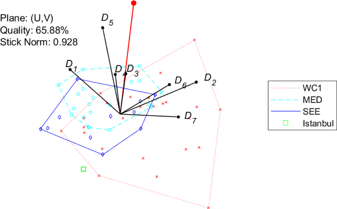
Figure 9 and Figure 10 show conjoint plots for the (overall 58) cities addressed in [9]-[11]: the three samples are distinguished, and referred to as MED, SEE and WC1, respectively. Note that the city of Istanbul, addressed both in Kılkış [9] and in Kılkış [10], is showed separately: this choice allows to point out more clearly the differences between the MED and SEE samples. To begin with, note that the representation of dimensions for both tools is very similar to the one obtained for the 120-city sample, as for the GAIA plane, also in this case the length of the stick is high (0.928) while the quality (65.88%) is lower than the one for the 120-city sample. As for the comparison of city samples, the following observations can be drawn:
MED and SEE samples (both located in specific geographical areas) are concentrated within relatively small areas of the plane, while the world cities in WC1 are spread in a larger area;
Overall, SEE cities have a slightly better index w.r.t. MED cities, while WC1 cities have a larger dispersion;
WC1 cities show a better performance in terms of social-cultural development (dimensions D2, D6 and D7) while MED (and up to some extent, SEE) cities are better in terms of energy systems and emissions (D1 and D5).
58 cities, GAIA: conjoint plot, distinguished samples
58 cities, Index/Dispersion: conjoint plot, distinguished samples
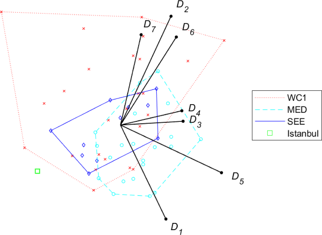
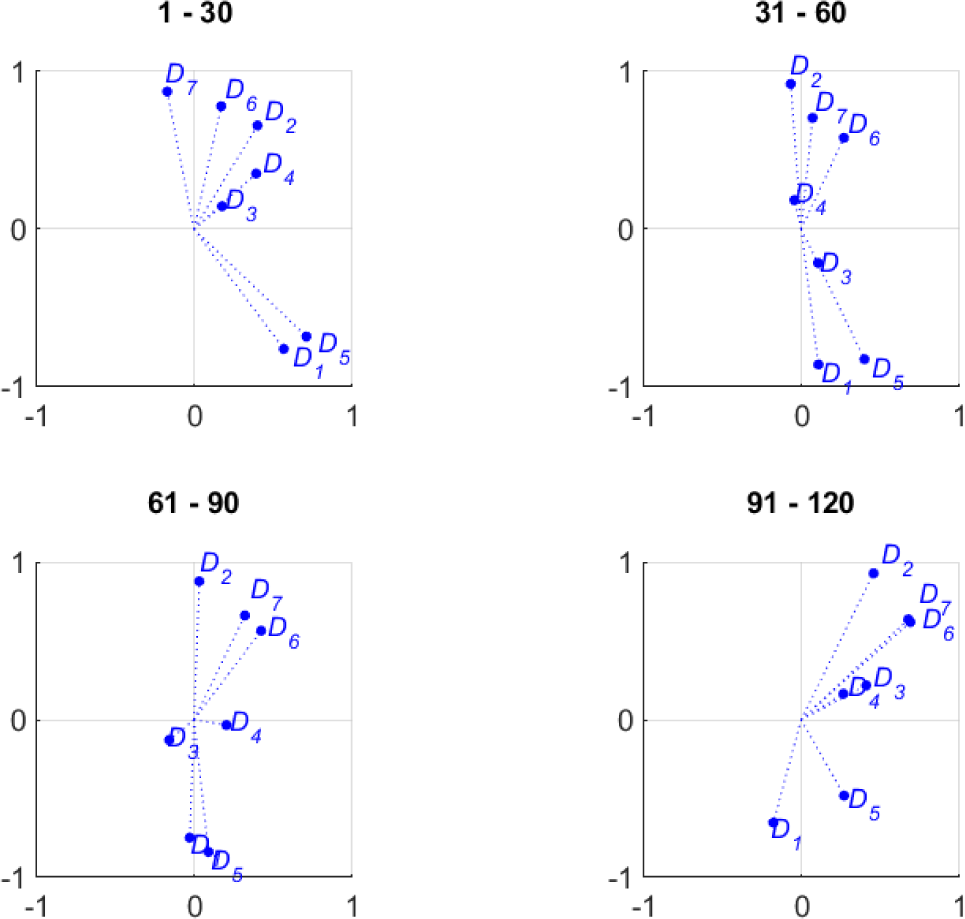
Figure 11 shows the criteria representations computed by the Index/Dispersion method separately for each quartile. The four plots show rather evident differences, following an apparent trend: roughly speaking, the pattern of criteria vectors seems to rotate clockwise from top to bottom quartiles. In particular, it is interesting to point out the behaviour of dimensions D1 and D5, that are closely related to a main focus of the SDEWES Index, namely the energy/emission decoupling. For the top quartile D1 and D5 have the strongest correlations to the index, meaning that they have the most relevant impact on the city ranking. This is consistent with the results in Kilkiş [5] (mentioned earlier in the present work) showing that the top ten cities propose best practices in energy saving and/or reducing emission. Moving towards lower quartiles, the role of D1 and D5 becomes less and less relevant, in favour of other dimensions, in particular D6 and D7. In the bottom quartile, D1 and D5 have the weakest correlation to the index, and are rather weakly correlated to each other. Overall, this behaviour seems to suggest that the leading cities are those that adopted integrated measures to reduce energy consumption and emissions at the same time, while for the less sustainable cities these two aspects seem to be rather disregarded, or at least, far from being addressed in a systematic way.
Index/Dispersion: criteria representation by quartile
The SDEWES Index is a tool for evaluating EWE systems, that are an inherently evolving objects. Faced with this fact, two attitudes are possible. One is to privilege adaptivity: conceive the index as a tool that is driven by the evolution (besides being itself, possibly, evolving) and thus continuously adapts its standards, renormalizing values to keep in line with the ongoing improvements. The other possible attitude privileges stability: conceive a tool that computes ranks uniformly along time, and thus can be used to track and measure the evolution. These two attitudes are both reasonable, but incompatible, and the goal of this work was not to take a stand, in the end, one may consider maintaining two (or more) different versions of the index. The goal of this work was to show that the adaptivity/stability dichotomy falls within the long-lasting debate about the relevance and legitimacy of rank reversal in the field of MCDA. Moreover, MCDA offers a viable (actually, the unique viable) approach towards stability. The SDEWES Index seems to be a rather good candidate in this sense. Clearly, devising an actual stable version of the index remains to be done. Similarly, it remains to understand whether, and up to what extent, the observations made on the SDEWES Index can be extended to other composite indexes, not necessarily limited to sustainability assessment.
As to the other contribution of this work, it has been shown that visual tools developed in the context of MCDA can be adapted to work in support of the SDEWES Index. These tools may be useful for analysis, to reveal information somehow hidden in the collected data, but also for dissemination, to enhance the comprehension of the scoring process and of its results. Here, in particular, the GAIA plane was adapted, and the Index/Dispersion plane was proposed. It has been shown that the two tools have similar expressive power, however, the latter is technically simpler and tailored to convey information relevant for the SDEWES Index. Clearly, further work on the Index/Dispersion representation is needed. To begin with, different measures of dispersion could be considered. Moreover, similar to the secondary planes in GAIA, further complementary views should be offered. To this aim, the proposed representation could be hybridized with projective (GAIA-like) techniques. Moreover, the Index/Dispersion method could be developed and generalized to work in a most general MCDA framework. Incidentally, this raises the question of how to consider data dispersion explicitly within an MCDA method, which may represent an interesting direction for research in the MCDA area.
This work has been partially supported by Research Project PRIN 2015 “Nonlinear and Combinatorial Aspects of Complex Networks”. The author is gratefully indebted to the anonymous Referees for the many constructive suggestions, that led to substantial improvements on the original manuscript.
- , 2012, http://www.unenvironment.org/resources/report/application-sustainability-assessment-technologies-methodology-guidance-manual-nov
- , https://ec.europa.eu/jrc/en/coin
- The Sustainable Cities Index, 2018, https://www.arcadis.com/en/global/our-perspectives/sustainable-cities-index-2018/citizen-centric-cities/
- Clean Air Scorecard ‒ A Clean Air Management Assessment Tool, http://cleanairasia.org/clean-air-scorecard/
- ,
Benchmarking the Sustainability of Urban Energy, Water and Environment Systems and Envisioning a Cross-sectoral Scenario for the Future ,Renewable and Sustainable Energy Reviews , Vol. 103 ,pp 529-545 , 2019, https://doi.org/https://doi.org/10.1016/j.rser.2018.11.006 - , 2016, https://digitalcityindex.eu/
- ,
European Digital City Index – Methodology Report, Nesta Report , 2016https://digitalcityindex.eu/ - , http://www.sdewes.org/sdewes_index.php
- ,
Composite Index for Benchmarking Local Energy Systems of Mediterranean Port Cities ,Energy , Vol. 92 (Part 3),pp 622-638 , 2015, https://doi.org/https://doi.org/10.1016/j.energy.2015.06.093 - ,
Sustainable Development of Energy, Water and Environment Systems Index for Southeast European Cities ,Journal of Cleaner Production , Vol. 130 ,pp 222-234 , 2016, https://doi.org/https://doi.org/10.1016/j.jclepro.2015.07.121 - ,
Sustainable Development of Energy, Water and Environment Systems (SDEWES) Index for Policy Learning in Cities ,International Journal of Innovation and Sustainable Development , Vol. 12 (1-2),pp 87-134 , 2018, https://doi.org/https://doi.org/10.1504/IJISD.2018.10009938 - ,
Benchmarking South East European Cities with the Sustainable Development of Energy, Water and Environment Systems Index ,Journal of Sustainable Development of Energy, Water and Environment Systems , Vol. 6 (1),pp 162-209 , 2018, https://doi.org/https://doi.org/10.13044/j.sdewes.d5.0179 - ,
Application of the Sustainable Development of Energy, Water and Environment Systems Index to World Cities with a Normative Scenario for Rio de Janeiro ,Journal of Sustainable Development of Energy, Water and Environment Systems , Vol. 6 (3),pp 559-608 , 2018, https://doi.org/https://doi.org/10.13044/j.sdewes.d6.0213 - ,
Data on Cities that are Benchmarked with the Sustainable Development of Energy, Water and Environment Systems Index and Related Crosssectoral Scenario ,Data in Brief , Vol. 24 , 2019, https://doi.org/https://doi.org/10.1016/j.dib.2019.103856 - , , Plenary Lecture at the 12th SDEWES Conference, 2017
- , , Multiple Criteria Decision Analysis: State of the Art Surveys, 2016
- ,
Multi-criteria Decision-making for Sustainable Metropolitan Cities Assessment ,Journal of Environmental Management , Vol. 226 ,pp 46-61 , 2018, https://doi.org/https://doi.org/10.1016/j.jenvman.2018.07.075 - ,
Operations Research for Sustainability Assessment of Products: A Review ,European Journal of Operational Research , Vol. 274 (1),pp 1-21 , 2019, https://doi.org/https://doi.org/10.1016/j.ejor.2018.04.039 - ,
A Review of Multi-criteria Assessment of the Social Sustainability of Infrastructures ,Journal of Cleaner Production , Vol. 187 ,pp 496-513 , 2018, https://doi.org/https://doi.org/10.1016/j.jclepro.2018.03.022 - , http://www. promethee-gaia.net/bibliographical-database.html
- ,
ELECTRE: A Comprehensive Literature Review on Methodologies and Applications ,European Journal of Operational Research , Vol. 250 (1),pp 1-29 , 2016, https://doi.org/https://doi.org/10.1016/j.ejor.2015.07.019 - ,
Analysis of the Potentials of Multi Criteria Decision Analysis Methods to Conduct Sustainability Assessment ,Ecological Indicators , Vol. 46 ,pp 138-148 , 2014, https://doi.org/https://doi.org/10.1016/j.ecolind.2014.06.011 - ,
On Rank Reversal in Decision Analysis ,Mathematical and Computer Modelling , Vol. 49 (5-6),pp 1221-1229 , 2009, https://doi.org/https://doi.org/10.1016/j.mcm.2008.06.019 - ,
On Rank Reversal and TOPSIS Method ,Mathematical and Computer Modelling , Vol. 56 (5-6),pp 123-132 , 2012, https://doi.org/https://doi.org/10.1016/j.mcm.2011.12.022 - ,
Visualization of a City Sustainability Index (CSI): Towards Transdisciplinary Approaches Involving Multiple Stakeholders ,Sustainability , Vol. 7 (9),pp 12402-12424 , 2015, https://doi.org/https://doi.org/10.3390/su70912402 - ,
Survey of Methods to Visualize Alternatives in Multiple Criteria Decision Making Problems ,OR Spectrum , Vol. 36 (1),pp 3-37 , 2014, https://doi.org/https://doi.org/10.1007/s00291-012-0297-0 - ,
Geometrical Representations for MCDA ,European Journal of Operational Research , Vol. 34 (1),pp 69-77 , 1988 - ,
Co-plot: A Graphic Display Method for Geometrical Representations of MCDM ,European Journal of Operational Research , Vol. 125 (3),pp 670-678 , 2000, https://doi.org/https://doi.org/10.1016/S0377-2217(99)00276-3 - , , Multicriterion Decision in Management, 2000
- ,
A Reconciliation Among Discrete Compromise Solutions ,Journal of the Operational Research Society , Vol. 38 (3),pp 277-286 , 1987, https://doi.org/https://doi.org/10.1057/jors.1987.44 - , http://www.promethee-gaia.net