Heat demand is seasonally oriented in heating networks, affecting the production of DH. DH systems usually have several production units, which are started based on their costs. This allows to divide the year into different time sets based on the production. The production data can be gathered into a duration curve, where distinct periods of production can be seen. The change in production scenarios affect the pumping areas since there is more energy to transfer and it is strongly affected by change in outside temperatures.

Usually DH systems have different pumping areas that serve the heat demand of buildings in that area. Whenever the heat demand changes, the production has to accommodate to this new demand by increasing or decreasing heat production and pumping power. This changes the balance of heat supply in the network.

To determine favorable locations for local production the network transfer of heat was simulated in different outside temperatures with a geographic information systems (GIS) model where every pipe, pumping station, production facility and customer DH substation have a geographical location. Also, the pipe characteristics are built into the model. This means that pipe size and length are also taken into consideration. The simulations were done with Trimble NIS. Trimble takes into account the DH pipe heat conductivity along with heat demand and outside temperature. For the calculations the Trimble program uses Neplan's heating basic module as a computing engine. [25]

The DH water temperature from the production facilities is based on the needs of the customers. Each customers DH substation has to have a certain DH water temperature in the corresponding outside temperature. The customer's geographical location set the need for certain temperature and flow from the production units. In this sense the customers on the edges of the network are critical in balancing the heat production.

The maximum potential for real estate owners to produce heat into the network was assessed with a calculator that optimizes the maximum heat pump installation (peak power) according to the profitability of the investment compared to real estate investor's return target. The size of the heat pump was calculated for each property type (retail, residential, logistics and office) and the heat consumption for each property type was the aggregated consumption of all buildings in the observed area. The consumption profiles were derived from real consumption data in the area weighting also for the building construction years.

The Heat pump sizing optimization follows the method presented by Kontu et al. [26]. In the method the current heat demand of a property (measured hourly over a year) is met with alternative heating solution (heat pump + electric boiler), and the size of the alternative solution is optimized so that the NPV of the investment is maximized. The annual net savings are calculated by deducting the costs of running the alternative solution from avoided DH costs. The paper presented the following formula (1) for the optimization.

$NPV=-(HP+EB+EC)+\sum _1^t\frac{{\sum }_1^{8,760}[H_{dh}\times P_{{dh}_t}-(\frac{H_{dh}}{COP}+H_{eb})P_{e_t}+H_{open}({P_{open}}_t-\frac{P_{e_t}}{COP})]+L_{{dh}_t}-OPEX-E_t}{{(1+r)}^t}$ (1)

Where HP, EB, EC are respective capital expenses for heat pump, electric boiler and larger electricity connection. The net savings from using heat pump is calculated with the following parameters: Hdh = consumed DH energy, Pdht = price (€/MWh) of DH at time t, Hhp = electricity required for HP, Heb = electricity required for EB, Pet= price of electricity, Hopen = energy sold to Open DH, Popent = price received for energy sold to Open DH, Ldht = load demand cost for DH, OPEX = operating expenses of HP, Et = fixed annual electricity capacity costs and r = used discount rate. A more detailed description of the method can be found in [26]. Since in this paper the heat that can be produced into the DH networks is analyzed more closely, the above method was altered so that the coefficient of performance (COP) changes when heat is produced into the network (in a higher temperature than needed for own consumption). Furthermore, basis scenario was calculated with one heat pump where if energy is produced into the DH network, the whole energy production for that hour is calculated with the lower COP (based on the DH supply water temperature). In the second scenario a second heat pump is installed (that increases the total capital expenses of the heat pump system by 25 %) that allows producing the first 50 °C of water with the higher COP and the rest with the lower COP (based on the supply temperature).

The DH system consists of several production units. There are two combined heat and power plants that have different production units. CHP 1 has one biofuel boiler and one coal boiler, each connected to their own steam turbine. There is also a gas turbine that is connected to a heat-recovery steam generator. CHP 2 has two waste-to-energy boilers that are connected to one steam turbine. CHP 2 also has a gas turbine that is connected to a heat-recovery steam generator. Both CHP plants also have heat storages that are used for balancing short term demand fluctuations. Heat only boilers (HOBs) are used whenever the heat demand is high or when a CHP plant is offline. The HOBs have gas as their main fuel and oil as a reserve fuel apart from HOB 2 that only uses oil. Peak power produced in 2018 was 654 MW and annual production was 1900 GWh. Length of the DH network was 564 km in 2018 [9]. More detailed information about the production units and the DH network is displayed in Table A1 (Appendix A).

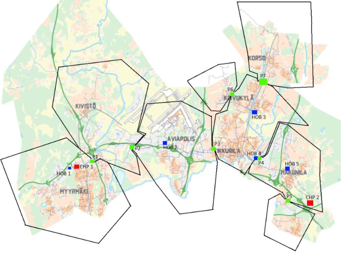
An overview of the district heating system and the location of the production units can be seen in Figure 1. The locations of the CHP power plants are marked with red squares (CHP 1 and 2), pumping stations in blue squares (P 1-7) and HOB's in green squares (HOB 1-5). The black lines mark the different pumping zones in the network.

Figure 1.

Overview of the DH network and production units

At every intersection of two pumping areas is a pumping station that has interchangeable pumping direction depending on the consumption and production of energy. The network is not built as a loop so the pumping areas do not change as the production is increased or decreased. However, some pumping stations are switched off when the production is decreased significantly in the summer and less pumping power is needed.

Simulation periods were determined according to the before mentioned method of analysing the changes in production over a year. During the year, three distinct periods of production were found. In one, during the coldest period of the year, all different production facilities are in use. In the second, only two main CHP plants are in use and in the warmest period of the year mainly one CHP plant is used. These three scenarios affect the pumping areas since there is more energy to transfer. The change in production occurs at outside temperatures of -26 °C, +0 °C and +14 °C. These are the three periods at which the DH network is examined more closely in the static network simulation. The duration curve can be seen in Figure A1 (Appendix A).

Validation of the simulation program was done in referencing the temperatures in the network given by the simulations to actual production temperatures from 2018 and the temperatures were during winter time. The result of this validation was that when temperatures were below freezing, the actual supply temperatures were between -4 % and +5 % of the value given by the simulation. In the summer time the temperatures were higher than in the simulation by about 10 %. This can be due to heat transfer to the neighboring cities that use a higher DH temperature.

The areas of interest can be seen in Figure 2. The temperature levels are indicated with colors blue, yellow and red. The temperature levels are different in each situation due to the different energy needs at that corresponding outside temperature. The temperature levels are <80 °C (blue), 80-82 °C (yellow) and 82-83 °C (red) when outside temperatures are +14 °C. In outside temperature 0 °C the same values are <91 °C (blue), 91-93 °C (yellow) and 93-94 °C (red). The values for outside temperature of -26 °C can be seen in Figure 3. The other two simulations can be seen in Figure A2 and Figure A3 (Appendix A).

Figure 2.

Areas of interest

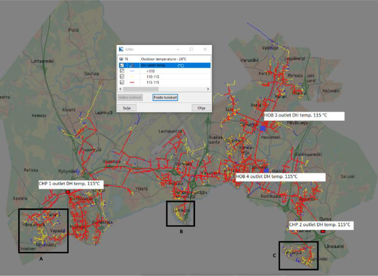
In all three simulations same locations appeared to have maximal decrease in supply temperature which would seem to make these areas favorable places for local production. These areas are marked as Zone A, Zone B and Zone C. These locations are, as expected, on the edges of the network, but surprisingly fairly close to the production units. Especially the southern areas of the network seem to be ideal for local production since these areas have larger parts of the network in lower temperature in the winter when heat is in high demand. The other parts of the network that have higher heat losses are usually due to longer transmission pipe to a neighboring network, a small industrial area or only a few consumers that are further from the main network.

One reason, according to Rämä et al. [27] for the drop in supply temperature could be low heat density in the depicted areas i.e. there is not much consumption in relation to the length of DH pipe. Especially when the heat consumption is very low in the summer, the flow of DH water in the pipes is also low. This leads to bigger heat losses in smaller pipes compared to large ones due to the smaller water volume. However, the increase in heat losses in the summer is a common problem for this type of heating networks in general. These areas offer an interesting possibility for the larger network if supply temperatures can be locally decreased, since this could give the possibility to decrease overall network supply temperatures.

The building stock of the areas presented in Figure 2 was analyzed in order to assess the potential for lowering supply temperatures. The collected building data is presented in Table 1. The zone with the largest building mass was zone A. This area also has the highest share of buildings that are not connected to the DH network. Zone A also has a fairly high share of residential buildings while there are also some retail and logistics buildings. Zone B has a more even division between residential buildings compared to other buildings and it also has the highest share of DH connected buildings. In zone C almost all of the buildings are residential buildings and the percentage of DH connection falls between the two other areas.

The improvement in energy efficiency of buildings has led to lower temperature needs on the secondary side temperatures (building side heating network). The recommended values reflect the buildings maximum values at the rated outside temperature of -26 °C for Southern Finland. For radiator heating for newly built buildings these are +45 °C and +30 °C degrees for supply and return temperatures respectively [28]. The values have drastically dropped from previous rated temperatures. However, the system must always be rated as low as possible without compromising indoor conditions. Rated temperatures for domestic hot water (DHW) heat exchangers are also presented, which are the same for all buildings. In the case heating network a minimum temperature of 65 °C is guaranteed to customers in order to achieve a DHW temperature of 58 °C. These values can be seen in more detail in Table A2 (Appendix A).

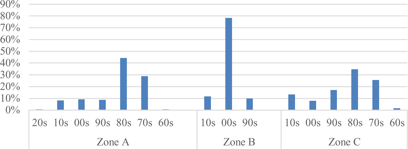
Since the construction year of the building affects the rated temperatures for the heating system, the year of connection to the DH network was also studied and can be seen in Figure 3. Zone A has the oldest connections. Zone B has the highest share of newly connected buildings while zones A and C are mainly connected in the 80s and 70s.

Figure 3.

Year of DH connection for studied areas

Based on these findings zone B, was taken as a priority due to newest buildings stock. Excess heat production potential is higher retail, logistics and industrial buildings than in residential and office buildings due to the lack of heat emitting processes in office and residential buildings. However, residential and office buildings can utilize heat pumps to recover waste heat from ventilation and waste waters. Commercial buildings can recover waste heat from cooling and other heat intensive processes.

The measured average temperature levels in the network vary between 76 °C and 109 °C on the supply side and between 29 °C and 51 °C on the return side. The absolute minimum temperature level in existing networks in Finland is defined by the heating of DHW which has to be 58 °C to avoid legionella bacteria. Lower levels are possible but require additional heaters on the DHW side. In addition, the flow restrictions of existing networks and customer heat exchangers limit lowering the temperatures at lower outside temperatures. Since the minimum temperature guaranteed in the existing network is 65 °C, this is taken as the lowest supply side temperature.

Reducing the supply temperatures in an existing DH networks has been widely recognized in Finland [29]. However, the progress seems slow even though newer buildings can utilize lower temperatures more efficiently as was also shown in the rated values of heat exchangers. The main issue is that normally networks contain new and old buildings in the same areas. However, areas of new buildings could be separated with a shunt connection or a heat exchanger to create new low temperature networks. Connecting a low temperature network to an existing network has been studied by Volkova et al. [30] on small networks. Dalla Rosa et al. studied separate low temperature networks (supply temperature 60 °C) with a shunt connection and found that a separate network was approximately 4 % more expensive compared to the more traditional network (supply temperature 90 °C), but due to lower operational costs, the end user tariff was almost the same [31]. Mostly due to long distribution distances in conventional DH networks the supply temperature has to be higher than the need of all customers to ensure the heat delivery for everyone in the network. This is one reason why low temperature DH networks need a separate connection to the conventional DH network.

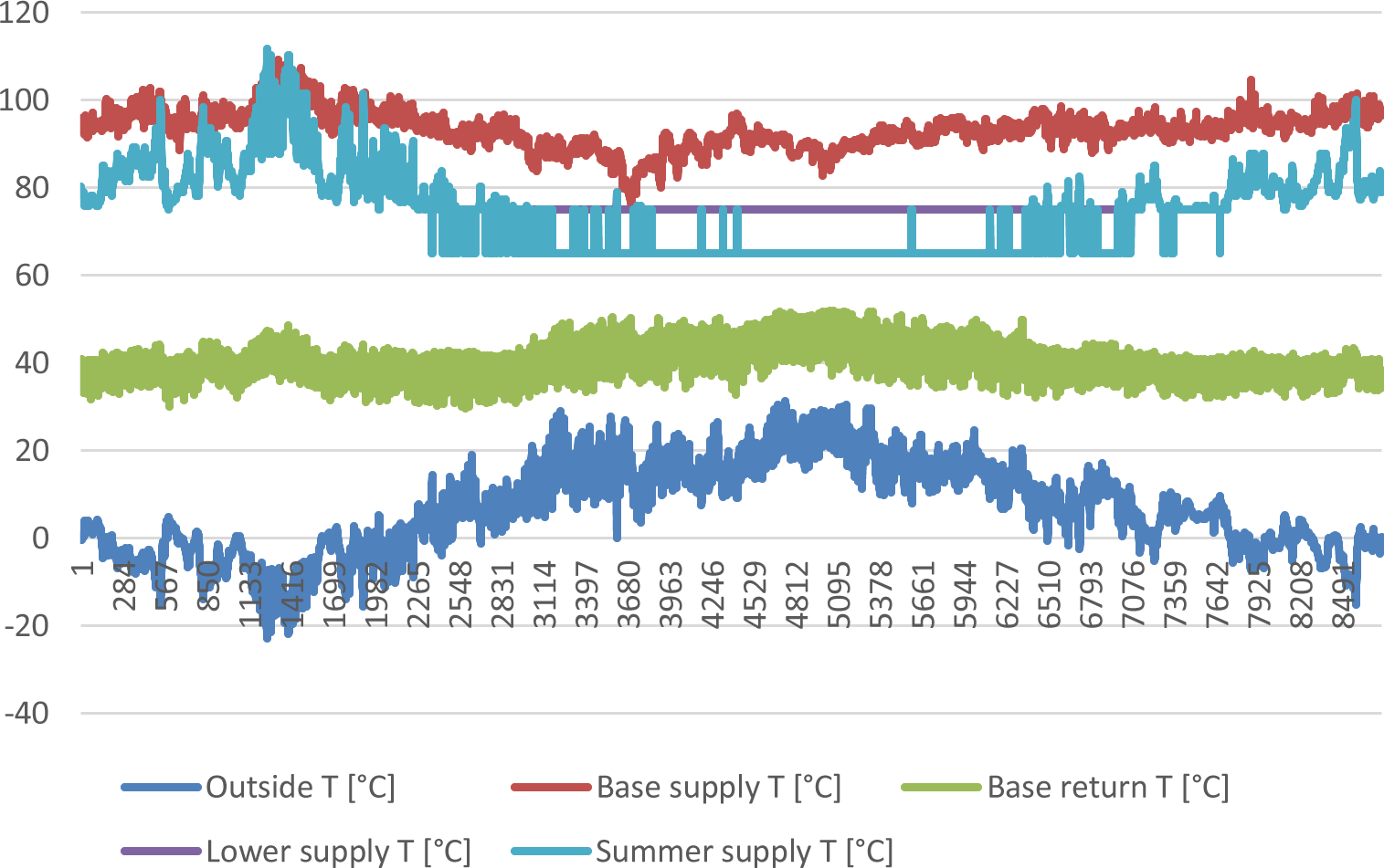
Comparing the actual supply temperatures to the recommended supply temperatures by the local energy company [32], it is estimated that supply temperatures can be decreased especially in the summer. In addition, since the minimum guaranteed temperature is 65 °C, the summer temperatures can be decreased further when temperatures are above 10 °C and heating is used only for DHW. These three different supply curves can be seen in Figure 4. These three scenarios are called Base, Lower and Summer. The return temperature was assumed to decrease the same amount as the supply temperature in Lower and Summer in outside temperatures below 5 °C compared to Base. In Lower at outside temperatures over 5 °C same return temperature was used as in Base. In Summer this was done at outside temperatures over 10 °C. The temperature levels can be seen in Figure 4.

Figure 4.

Supply temperature curves

The simulation results were earlier presented in Figure 3. In closer inspection of the marked areas the heat load and losses were simulated with Trimble. The simulation results can be seen in Table 2, where zone A is the western most area in the network. Correspondingly zone B is in the middle and zone C in the east.

The simulation was verified regarding Zone B with actual consumption data from 2018. The actual measurement data corresponds well to the simulation results.

The amount of local heat pump production increased in all real estate types as the supply temperature decreased being at maximum 1214 MWh or 4,6 % of the total annual heat consumption. The results of the heat pump investment optimization are presented for all real estate types in Table 3.

Already at current temperature levels investments into local heat production would be reasonable with a total amount of production being 145 MWh with a single heat pump installation. Production in total increased 782 % compared to Base scenario using temperature levels from Lower scenario. This increase was 839 % compared to Base scenario using temperature levels from Summer scenario. These increases were similar with installations of two heat pumps but the total produced energy was smaller.

In terms of excess heat production and profitability in all real estate types, the production system with one heat pump appears to be better. This is due to the smaller investment. The largest potential of excess heat production was in retail buildings.

The heat pump production was largest in winter between November and February most likely due to higher prices paid for the surplus heat coinciding with low electricity prices. However, this is beneficial for the DH system, since heat demand is largest in the winter. The optimization results are displayed in more detail in Table A4, Table A5, Table A6 and Table A7 (Appendix A).

Hourly heat losses were estimated based on the network information using the actual supply and return temperatures. The change in heat losses were assessed with a network model consisting of actual network data on pipe dimensions and lengths. The values used in the heat loss calculations can be seen in Table 4. The reduction in heat loss was significant decreasing 16.6 % and 22.1 % in the two studied cases compared to the current base scenario.

The reduction in heat loss and local production also reduces emissions from the overall heating system. Heat loss reduces the need for all production, but it is assumed to decrease DH production. The local heat pump production also replaces DH production but causes emissions because of increased electricity use. However, this will reduce overall emissions because of heat pump efficiency and smaller emission intensity of electricity. Emissions reduced due to smaller losses were 82 498 kg_CO² and 109 421 kg_CO² in scenarios Lower and Summer respectively. The maximum emission reduction from excess heat production was 170 020 kg_CO² in Summer scenario with one heat pump installation. The total emissions of the area in Base case were 7 085 269 kg_CO² so the overall emissions reduction from reduced losses and excess production was 4 %. Emission factor for produced district heat in 2018 in Vantaa was 247 g_CO²/kWh [33]. The increased electricity consumption of heat pumps was calculated with an emission factor of 107 g_CO²/kWh [34].

Also overall production cost is likely to decrease even though the prosumers are compensated from their production if the pricing of excess heat from prosumers is correctly priced from the energy producer. However, this aspect was not thoroughly investigated in the article.