


Transportation sector currently consumes about 20% of globally produced fossil fuels [1], thus making it the second largest carbon dioxide (CO2) emission source [2]. According to the study presented in Jiang and Guan [3], this trend is most emphasized in the developing world, where inland transportation represents a major contributor to the total CO2 emissions balance. One way of dealing with the problem of transportation system energy efficiency and Greenhouse Gases (GHG) emission issues, would be through improved advanced transportation policies promoting Intelligent Transportation Systems (ITS) and multi-modal transport and greater inclusion of railways in the overall transportation mix [4], with electrified urban public transport in particular identified as key technology for achieving the goal of cleaner air in urban environment [5]. The aforementioned facts also represent the key motivation for systematic electrification of the transportation sector and phasing out of fossil fuel sources [6], which has been most emphasized in road transport applications through introduction of hybrid electric and fully-electric vehicles [7], whose optimal charging represents one of the key issues in the concept of the smart grid [8]. However, rather high capital railway infrastructure electrification costs currently prohibit the full electrification of long railway lines in Europe with low traffic volumes [9]. Hence, for the time being, rail transport on these routes needs to be covered by diesel-powered locomotives, whose utilisation can be foreseen for at least thirty more years [10].
In order to tackle the problem of railway transport energy efficiency, introduction of energy storage technologies has shown great potential, as shown by the study presented in Ovalle et al. [11]. This approach can also be employed with diesel-electric locomotives in order to improve their energy/fuel efficiency and to achieve the GHG reduction goals through hybridization of diesel-electric locomotive powertrains by means of adding a suitably sized battery energy storage system [12]. Alternative energy storage technologies suitable for railway vehicle hybridization have also been considered in the literature. These included flywheels [13], hydro-pneumatic energy storage systems and ultracapacitors [14], but are typically limited in energy storage capacity, and can primarily be used for railway train kinetic energy harvesting during braking over relatively short distances. Moreover, it should be noted that energy consumption and GHG emission optimization in rail transport represents a multi-dimensional nonlinear problem characterized by numerous technological and traffic limitations [15]. One such study has been carried out in Cipek et al. [16], and has shown remarkable potentials for fuel efficiency improvement and GHG emissions reduction (over 16% improvement) compared to the traditional diesel-electric locomotive benchmark case for a quite demanding mountainous rail route. However, when analysing the financial benefits of diesel fuel savings, one may also need to consider the realistic diesel fuel expenditures, which entails a detailed analysis of well-to-wheel fuel costs, such as the one presented in Li et al. [17].
The second crucial aspect of rail transport is its timely scheduling and safety, which may be further emphasised if autonomous railway vehicles are concerned [18], which represents a key long-term development issue for associated industries [19]. In that respect, Matsumoto and Kitamura [20] presents an autonomous distributed train scheduling system within which locations and speeds of particular trains are communicated to the centralised database. Based on these data, the central dispatching system can optimise the traffic flow and improve the rail route throughput. Obviously, accurate localisation and real-time speed estimation of individual traffic entities and traffic flow in general is crucial for the operation of such systems [21], wherein Talvitie et al. [22] proposes utilisation of fifth-generation (5G) New Radio (NR) networks. These communication systems may be additionally augmented with advanced remote sensor fusion techniques, such as those based on Extended Kalman Filter (EKF) approach [23] in order to obtain precise real-time information on position and speed of high-speed trains. In fact, limited bandwidth and data throughput, along with perceptible data transfer latencies of Global System for Mobile Communications – Railway (GSM-R) systems makes them increasingly difficult to accommodate high-speed trains, thus motivating a transition to 5G communication networks [24]. Standardisation of high-speed train communications, as indicated in Hasegawa et al. [25], can facilitate novel technologies capable of supporting future railway Information and Communication (ICT) systems [26], including Internet of Things (IoT) [27]. Hence, increased influx of Industrial Internet of Things (IIoT) technologies [28] into the transportation sector can be anticipated as well as other sectors, such as smart grids [29]. Ultimately, 5G communication systems can also be used to further propel intelligent railway transportation technologies [27], as well as dedicated cloud-based services aimed at transportation energy efficiency improvement [30], and increased freight rail transport safety through introduction of on-board distributed sensor networks [31]. In that respect, 5G communications networks enable ‘cross-industry’ solutions important for integration of traffic systems other industrial or public systems [32]. Therefore, the new Radio Access Network (RAN) design and 5G systems’ high localisation precision and availability are crucial for advanced traffic systems and future inclusion of the so-called ‘telematic’ interfaces for the remote notification and advising of the train driver, as well as precise positioning of high speed rail vehicles [33]. These systems may be able to supply the precise information to autonomous trains where the minimum requirements for availability can be as high as 99.9999% [22]. On the other hand, 5G technologies can be used for narrow-bandwidth communication with remote sensors networks for aiding rail vehicles by providing warnings about potential problems at the track more reliably than earlier-generation communication systems. Thus, novel 5G narrow-band communications open new ways to increase the traffic safety through increased vehicle autonomy [34], while simultaneously having virtually no maintenance requirements over the anticipated ten-year exploitation period [35].
Finally, weather conditions are crucial for railway transportation safety [36], because they effectively determine [37]:
Visibility in case of rain, snow, sleet or fog;
Track-to-wheel adhesion deterioration due to snow or ice;
Head wind-related air-drag;
Otherwise hazardous traffic conditions, for example in the case of sudden flash floods.
Moreover, in the case of passenger transport, weather conditions may also affect the passenger flow, wherein temperature and precipitation may result in increased number of passengers per train [38], whereas the increase in wind may have an opposite effect [39]. Therefore, it would be advisable to provide real-time weather and rail track conditions to the driver and the dispatch centre [40]. In this way, an optimal driving strategy can be devised, or the scheduled train departure may be postponed until favourable conditions are met. Simulation models which include realistic rail track profile [41] and information about adhesion limits [42] may provide the dispatch centre with additional information which may crucial in the decision-making process.
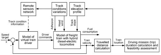
Based on the available literature review, it appears that none of the listed works have considered a systematic approach to simultaneous the energy efficiency performance assessment and safety indices analysis, which are both crucial for the future of railway transportation. Moreover, integration of advanced wireless communication technologies may provide a certain advantage in terms of timely access to critical information about track conditions, thus providing additional means of transportation system performance optimisation. Having this in mind, the hypothesis of this paper is that by utilizing advanced fast-throughput remote sensor networks for timely information on weather conditions related to track adhesion and head wind, the performance of a freight train equipped with a hybrid locomotive and travelling over a mountainous region characterized by notable gradient variations can be adjusted so that it may complete the task while maintaining favourable energy efficiency indices. The main novelty of this paper is in a systematic approach to building of a simulation model of track condition information exchange within the distributed remote sensors network, and its integration with the model of a freight train powered by a hybrid diesel-electric locomotive previously developed in Cipek et al. [16] for the purpose of energy efficiency and train driving mission safety assessment over a particular mountainous railway route. The overall model has been implemented within Matlab/SimulinkTM software environment. Based on the results presented in this work, recommendations useful for planning of train missions are also given. The key aspects of the presented research methodology are illustrated by the flowchart in Figure 1.
Principal block diagram (flowchart) of proposed methodology for railway train fuel efficiency and safety assessment
The paper is organised as follows. Section 2 presents the sub-models of the railway train travelling over a mountainous railway route, which include the railway route elevation, track adhesion and head wind profiles, models of hybrid diesel-electric locomotive power-train and battery energy storage system, and train driver model. Section 3 outlines the model of a narrow-band distributed remote sensor network based on 5G mobile technology and its integration with the freight train model in terms of data exchange. Section 4 presents the simulation results of the proposed freight train model augmented with real-time remote sensor data under varying track adhesion and head wind conditions, along with the assessment of energy efficiency and safety improvements. Concluding remarks are given in Section 5.
This section outlines the mountainous railway route from Cipek et al. [43] and the hybrid diesel electric locomotive model developed in Cipek et al. [43] based on a suitable conventional diesel-electric locomotive [44], wherein identical driver command interface adopted from Valter [45] is used. The hybrid locomotive model also utilises the optimised energy management control strategy developed in Cipek et al. [16].
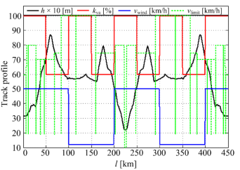
Main characteristics of the mountainous rail route between the towns of Oštarije and Knin (Lika region, Republic of Croatia) in terms of elevation profile and speed limits are illustrated in Figure 2, wherein black curve represents the route elevation profile (h), while green dashed trace represents railway train speed limits (vlimit). These traces were defined in Cipek et al. [43] using free on-line Global Positioning System (GPS) Visualizer utility software [46] and an on-line source for the particular track speed limitation [47], respectively. Additional information in Figure 2 is related to the relative adhesion coefficient (kva), (ratio of available adhesion with respect to the nominal case), whose availability is assumed based on the remote sensors grid data (see discussion in subsequent sections). In particular, the presented relative adhesion coefficient values roughly correspond to dry track and wet track adhesion conditions. Since the variable adhesion (wheel-to-track friction) coefficient (μa) within the freight train model can be expressed by multiplying the theoretical result from Pichlík and Zděnek [48] with the relative adhesion coefficient kva, this results in the following adhesion coefficient expression:
(1)
with μmin = 0.161 representing the adhesion coefficient minimum value, and other velocity-related constants parameterised as β = 7.5 km/h and γ = 44 km/h according to Pichlík and Zděnek [48].
Finally, blue curve in Figure 2 represents the average wind velocity (vwind) profile, which is also assumed to be available from the distributed remote sensors grid (see subsequent sections). According to Valter [45], this additional relative wind velocity affects the specific motion resistance (wk0) [N/t]. Due to the same train configuration from Cipek et al. [16] used in this paper, a specific motion resistance for heavy cargo trains can be defined as:
(2)
Note that the minimum value of wind velocity addition vwind is 12 km/h (Figure 2), which is according to Valter [45] a commonly used value within the above wind resistance model.
Altitude, traction coefficient, head wind speed, and train speed limit profiles for the rail route considered in this work
According to Valter [45], the train movement is also subject of the railway track curvature radius effects and track gauge. For the sake of simplicity, an equivalent constant-valued average curvature resistance ( [N/t]) is adopted herein, as proposed in Cipek et al. [16].
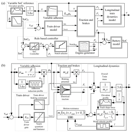
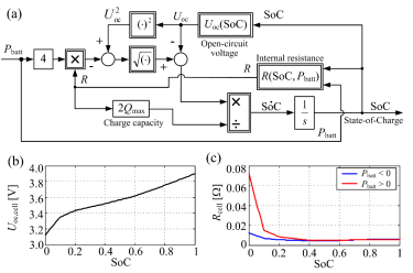
Figure 3a shows the overall quasi-steady-state model of the battery-hybrid locomotive [16], comprising the train driver, longitudinal dynamics, electrical traction and mechanical brake system sub-models (framed by dashed lines), which are given in more detail in Figure 3b. The power-train sub-models are modelled by means of static characteristics (maps), which are originally developed in Cipek et al. [16].
The driver model subtracts the freight train model velocity (v) from the velocity reference (target) (vref), and the resulting difference is used to generate the train driver control output in terms of throttle ‘Notch’ position and braking ‘Brk’ commands. These are partitioned into eight positive ‘Notch’ levels corresponding to constant traction power operation, one zero-valued neutral ‘Idling’ position, and eight negative ‘Notch’ levels for regenerative braking at constant braking power [16]. The driver model is configured as a simple proportional term with gain (KDr) [16], and its output is subsequently quantized resulting in seventeen integer values related to ‘Notch/Idle/Brk’ commands, and also saturated so that the ‘Notch/Brk’ command selection does not exceed the definition range from –8 to +8 (Figure 3b) [43]. In the case of deceleration, additional braking action by means of mechanical brakes can be applied if train velocity exceeds 1 km/h over the targeted value, i.e., when regenerative braking cannot effectively dissipate the train’s kinetic energy (i.e., at low train longitudinal speeds). The combined braking command ‘Brk’ (utilising traction system regenerative braking and mechanical brakes in Figure 3a) also takes into account the wheel vs. track braking potential [16].
Block diagram of battery-hybrid locomotive model (a) and electrical traction sub-model (b)
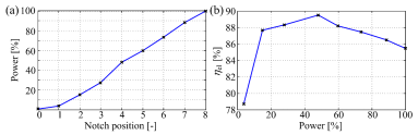
Percentage of maximum electrical traction power (Pt,max = 1,402.08 kW [43]) at each ‘Notch’ position is shown in Figure 4a, whereas Figure 4b shows the overall efficiency of the electrical traction system ηel(%P) as a function of the percentage of nominal power. The traction force (Ft) based on the ‘Notch’ position-related engine-generator set power output, traction system overall efficiency and train velocity v as follows [16]:
(3)
where v is the locomotive (and train) longitudinal velocity given in km/h, %P(Notch) is the electric power percentile of ‘Notch’ position and Pt,max [W] is maximum locomotive power. The traction power is included within the model as a static map [16], utilising the train velocity and ‘Notch’ as inputs to calculate the electrical transmission power (Pt).
Locomotive power production vs. ‘Notch’ command (a) and overall electric power conversion efficiency curve (b) [43]
Maximum traction force is also limited by the maximum wheel vs. track adhesion characteristic, as discussed above. This, in turn, is limited by the normal force exerted by the locomotive weight ml × g according to the following expression:
(4)
where α is the track slope, typically within ±2.5 degrees (thus the approximation cosα ≈ 1 is valid in this case). Note that, in the case when conventional brakes are applied overall train weight is taken into account for maximum braking force.
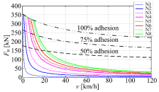
Hence, the maximum traction force can be obtained by combining eq. (3) and eq. (4) utilising the overall hybrid locomotive weight (ml = 107.85 t [16]). These traction force curves for each ‘Notch’ are shown in Figure 5, wherein negative wheel-to-track force values are obtained for the case of regenerative braking. Figure 5 also shows the maximum locomotive traction for 100%, 75% and 50% of adhesion, which illustrates that the variable adhesion effect to traction characteristic is dominant in low-speed high-power operating regimes.
The sub-model for longitudinal motion in Figure 3b represents the simplified dynamics of a lumped overall mass of the train (ma) [kg] subject to locomotive traction and total braking forces Ft and Fb, respectively, along with aerodynamic drag and rolling resistance forces, and the overall gravity force component ma × g × sinα due to the track slope. The final model is given by Valter [45]:
(5)
Maximum traction force vs. velocity curves with ‘Notch’ command and wheel-to-track adhesion as parameters
In the above eq. (5), wk and wr [N/t] are the specific resistance coefficients corresponding to air drag and curvature motion, respectively. In the proposed model, traction and braking forces Ft and Fb are affected by adhesion and head wind variations (simulated through varying the relative adhesion coefficient kva and head wind velocity vwind, as shown in Figure 2). These adhesion and head wind variations are assumed to also be available to the driver from the remote sensors measurements.
The traction power is also included as a static map [16], and uses the same train velocity and ‘Notch’ inputs for the electrical transmission power Pt calculation. The difference between transmission power Pt and generator power (Pg) feeds the battery model directly over the common Direct Current (DC) link. The battery energy storage model is derived in Bin et al. [49] from the battery equivalent electrical circuit, and is presented in Figure 6a (note that positive values of battery input power (Pbatt) correspond to battery discharging operation). For the particular battery model, characterised by State of Charge (SoC)-dependent open circuit voltage (Uoc) and internal resistance (R) (with the internal resistance also being dependent on current/battery power sign), the parameters of a single Li-Ion battery cell have been adopted from Autonomie software, and are shown in Figure 6b and Figure 6c. Battery sizing has been performed in Cipek et al. [16] and results in 900 kWh of total battery energy storage system capacity (arranged in 75 parallel modules comprising 200 series-connected cells each), which is characterised by the overall battery system weight of 9,450 kg [16].
A rule-based controller shown in Figure 3a (also developed in Cipek et al. [16]) uses the transmission power demand Pt and the battery SoC controller power demand (PbR) to calculate the power required from the main engine-generator (PgR), and, subsequently the required throttle NotchRB by means of the ‘Notch’ selector map. In the case when the requested power PgR is lower than the power generated when NotchRB = 4 is selected, low-efficiency operation of the engine is avoided by bringing it to idling ([16]) to avoid the highly-impractical engine on/off operation. The engine-generator sub-model provides the fuel and emission rates and the electricity generator power output Pg for each NotchRB as shown in Table 1.
Battery power flow model (a); cell open-circuit voltage vs. SoC (b) and cell internal resistance vs. SoC and current sign (c)
Hybrid-electric locomotive diesel engine and generator set data from Cipek et al. [16]
| Throttle position | Main engine power Pmg [kW] | Generator power Pg [kW] | Fuel rate [g/s] | Emissions rate [g/s] | |||
|---|---|---|---|---|---|---|---|
| Hydrocarbons (HC) | Carbon monoxide (CO) | Nitrogen oxides (NOx) | CO2 | ||||
| IDLE | 6.43 | 0 | 2.5704 | 0.0299 | 0.0436 | 0.1510 | 7.9910 |
| Notch 4 | 632.77 | 566.49 | 40.8315 | 0.0834 | 0.1503 | 2.4458 | 129.3824 |
| Notch 5 | 787.15 | 694.13 | 51.6475 | 0.1136 | 0.3057 | 3.2341 | 163.4197 |
| Notch 6 | 965.83 | 844.70 | 64.2834 | 0.1593 | 0.9703 | 4.0096 | 202.2778 |
| Notch 7 | 1,161.70 | 1,004.73 | 79.8195 | 0.2585 | 2.2294 | 4.8944 | 249.5078 |
| Notch 8 | 1,312.80 | 1,121.67 | 94.4690 | 0.3314 | 4.1517 | 5.2350 | 292.7589 |
The battery charging/discharging power demand is commanded by the proportional-type SoC controller (Figure 3a), characterised by its gain (KSoC) and a dead-zone (ΔSoC) to avoid controller output ‘chattering’ when the control error signal eSoC = SoCR – SoC is near zero. Cipek et al. [43] suggested that it would be convenient to use a variable SoC reference due to mountainous route being characterized by significant variations in elevation profile resulting in notable variations of train potential energy. This approach is also used based on the known lowermost and uppermost elevation levels hmin and hmax as input parameters [43]:
(6)
with SoCbl and SoCbh representing the minimum and maximum values of the variable battery SoC target.
In this study, the SoC controller parameters (KSoC, ΔSoC, SoCbl, SoCbh) have been obtained by using a DIviding RECTangles (DIRECT) search-based optimisation [50], aimed at minimising the overall locomotive fuel consumption for two different simulation scenarios, subject to the minimum battery SoC constraint of 20% and without considering battery aging effects over a single train driving mission. The first scenario corresponds to a fully-loaded train (630 t of cargo hauled by the locomotive [43]) and constant wind velocity of 12 km/h and 100% adhesion, representing the nominal (benchmark) case herein. The second scenario corresponds to variable adhesion and wind velocity profiles from Figure 2. Each optimisation run performed for the particular train load results in a unique set of locally-optimal SoC controller parameters listed in Table 2.
SoC controller parameters for different hybrid locomotive operating modes
| vwind and kva | Parameters | |||
|---|---|---|---|---|
| KSoC | ΔSoC [%] | SoCbl [%] | SoCbh [%] | |
| Constant | 12,055 | 4.32 | 42.16 | 52.32 |
| Variable | 1,006 | 1.46 | 42.34 | 56.37 |
This section presents a simulation model of a narrow-bandwidth distributed sensor network based on 5G mobile technology, which is integrated with the previously described battery-hybrid locomotive-based freight train model, and thus-obtained overall model is also equipped with a visualisation interface.
According to Figure 5 and the related discussion presented above, the auxiliary variables needed for the effective operation of the freight train traction control system and battery SoC controller are those related to track conditions, i.e., the wheel vs. track adhesion potential and head wind, which directly affect the wheel traction and train motion resistance. These track-related variables are directly related to atmospheric conditions, in particular temperature and air humidity are related to wheel traction [coefficient μa in eq. (4)], whereas wind speed and its direction (head wind) define the additional motion resistance according to eq. (5). Hence, the aforementioned atmospheric variables need to be measured by an array of remote sensors and periodically transmitted to a server comprising a central database which the train driver would access in order to receive the most recent track condition updates in order to adapt the train control strategy.
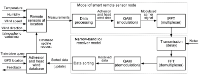
Figure 7 shows the block diagram representation of Narrow-Band (NB) IoT remote sensor node connection to a central database containing track adhesion and head wind data from a remote sensor network distributed equidistantly along the railway track. The remote sensor node model comprises the physical sensors (transducers) of air temperature and humidity, and wind speed and direction (atmospheric variables), whose measurements are processed in order to obtain useful information about track condition (i.e., adhesion and head wind). These data (digital information) is prepared for radio transmission by means of Quadrature Amplitude Modulation (QAM) of the carrier signal ([51]). This is a form of Orthogonal Frequency Division Multiplexing (OFDM), typically used in Long Term Evolution (LTE) or 4G communication networks [52]. In order to convert the parallel QAM data output into radio signals suitable for transmission, Inverse Fast Fourier Transform (IFFT) [53] is used within this framework. Signal transmission from the sensor node to the NB IoT receiver model can be emulated by a transport delay (and, possibly, by an external noise source). At the receiver side, the modulated radio signal features are extracted by means of Fast Fourier Transform (FFT) [53], which are subsequently passed to the QAM demodulator for the extraction of useful data. The extracted data is sorted (indexed) before being stored in the central database which may be updated periodically or upon the train driver’s request with the track condition data relevant for the particular geographical location (characterised by its GPS coordinates).
Block diagram representation of NB IoT remote sensor node connection to central track adhesion and head wind database
This section presents simulation results for the hybrid diesel electric locomotive driving mission over the selected mountainous route. The model is simulated with variable adhesion and wind velocity profiles and compared with results derived by constant commonly used values of aforementioned parameters in order to get insight how optimised set of controller parameters can affect the battery SoC and fuel consumption.
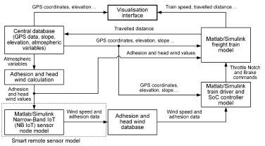
Figure 8 shows the integration of the freight train and driver (control strategy) sub-models with the geographical railway route sub-model and the remote sensor network model, wherein individual model components are implemented within Matlab/Simulink software environment [54].
The freight train simulation model is fed rail track elevation and slope data from GPS coordinates (geographical data) from the general database which also contains the corresponding set of atmospheric variable data for each geographic location. In this way, all parts of the simulation model receive relevant data, which is updated based on the distance travelled by the train along the railroad track. The same geographical data is also fed to the driver model (and the battery energy storage system SoC control strategy) for the purpose of energy consumption optimisation (see previous chapter). Based on the train geographical location (position along the rail track), relevant remote sensor data corresponding to traction adhesion potential and head wind is selected and used within the driver model in order to select appropriate throttle ‘Notch’ (or ‘Brk’) command in order to maintain the train motion (to avoid wheel slipping). The same data is also used within the freight train model to emulate the realistic wind resistance (drag) and traction force potential variations with changes in adhesion characteristics.
Finally, the overall simulation model also comprises a visualisation interface which can be used for online monitoring of key freight train variables (such as speed, travelled distance, traction force and others).
Block diagram representation of integrated simulation model comprising freight train and driver, smart remote sensor node and track data exchange sub-models
Train driving simulations are conducted for the round trip over the mountain route characterised by the elevation profile shown in Figure 2, wherein the locomotive hauls 630 t of cargo wagons (roughly corresponding to the maximum load of a single locomotive over that particular route, as indicated in Škrobonja et al. [44]). Simulations are carried out within Matlab/SimulinkTM software environment. Figure 9 shows the throttle ‘Notch’ and braking ‘Brk’ commands wherein the blue trace marked (Co) represents the scenario where constant (benchmark) values of wind velocity and adhesion are used (vwind = 12 km/h, kva = 100% [16]), while the red trace marked (Vo) corresponds to the scenario with variable values defined in Figure 2. The results in Figure 9 also indicate that over that route electrical (regenerative) braking is not always sufficient, thus mandating utilisation of additional mechanical (friction) brakes, in particular during train descending from higher elevation (Figure 9 and Figure 2).
Train driver commands
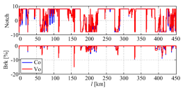
Figure 10 shows corresponding train velocity over travelled distance and time. Using a-priori known train speed limitations (Figure 2), the train speed target vref (black trace in Figure 10a) emulates the train driver behaviour who would gradually increase and decrease the ‘virtual’ train from one to another speed limitation value. Such train speed target generation is performed herein over a 2 km window, as indicated in Cipek et al. [16]. For the given speed target vref and constant values of vwind and kva, the actual train velocity (vCo) for the nominal (benchmark) case is obtained in simulation and represented by the blue trace in Figure 10, while the red trace represents the actual train velocity (vVo) when variable values from Figure 2 are used. The difference in velocities of the aforementioned driving scenarios is not emphasized, as shown by spatial speed traces (i.e., speed vs. the travelled distance) in Figure 10a. However, when these velocity traces are plotted vs. the elapsed driving mission time (Figure 10b), the considered simulation scenarios are characterised by different driving mission durations. This indicates that the proposed simulation model also may be helpful for the prediction of possible train delays for the a-priori known rail track adhesion and head wind conditions. As expected, adhesion below nominal value and head wind increase deteriorate the locomotive traction performance and result in lower train speeds, especially during ascending phases of the journey, which results in lower train velocities and slower driving mission completion (Figure 10b). It should also be noted that in the case of notable upward track slope, the freight train velocity profile following performance would also be deteriorated, especially when adverse track conditions are present. Namely, in those cases the electric motor-based traction system cannot provide enough traction action in order to keep the train velocity close to the target value, which is manifested in lower train velocities than the speed limit for the particular track segment. Thus, the track slope effect also contributes to the prolonged duration of the driving mission and its completion.
Train velocity over distance (a) and over time (b)
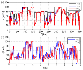
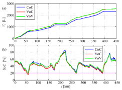
Figure 11 shows the locomotive fuel consumption and battery SoC for three different scenarios concerning a battery-hybrid locomotive:
Constant vwind and adhesion kva (benchmark case) are used in simulation and controller parameters are optimised for these constant parameters (CoC scenario), which directly relates to the main optimisation result presented in Cipek et al. [16];
Variable vwind and adhesion kva are used in simulation, while the control strategy parameters are derived for benchmark values (VoC scenario);
Variable vwind and adhesion kva are used in simulation, and the control strategy parameters are optimised for these variable track parameters (VoV scenario).
Figure 11a shows that the fuel consumption traces, while Figure 11b shows the SoC traces for the considered CoC, VoC and VoV scenarios. The benchmark CoC scenario originally presented in Cipek et al. [16] is, unsurprisingly, characterized by the lowest fuel consumption result, while also maintaining the battery SoC above the minimum recommended value (SoCMIN = 20%). The aforementioned fuel consumption ‘optimality’ of this benchmark case is primarily related to the absence of adhesion variability which enables the locomotive powertrain to utilize the regenerative braking potential for battery recharging to its full extent. In the VoC case, battery SoC exhibits deeper discharges (SoC falls below 20%) compared to the cases of CoC and VoV target. Namely, in the cases of CoC and VoV scenario, the optimised SoC controller parameters are derived subject to the minimum battery SoC constraint of 20%. In this way, by using data from remote sensors grid of track conditions, and properly optimised control strategy parameters, deep battery discharging is effectively avoided. This would in turn result in less emphasised aging of the battery pack, and, consequently, in extension of battery cycle and calendar life compared to the case when no such measures could be applied. In all of the aforementioned cases, battery SoC profiles are highly reminiscent of the actual railway track elevation profiles (Figure 2). In particular, the positive (rising) SoC trends are associated with downward track slopes characterised by extensive utilisation of regenerative braking via the electric traction system, whereas the negative (falling) SoC trends are associated with upward track slopes mandating additional utilisation of battery power (battery discharging operation) for improved traction performance. The fuel consumption data in Figure 11a indicates that VoC and VoV scenarios are characterized by noticeable fuel consumption increase over the CoC case. Final values (VfCoC = 2,320 L, VfVoC = 2,552 L, VfVoV = 2,556 L) confirm that track conditions variability (i.e., variable head wind and traction coefficient) may yield up to 10% higher fuel consumption, which is caused by the increased drag due to additional variable wind velocity combined with less available regenerative braking power when adhesion is decreased. VoV scenario shows that that the locomotive consumes negligibly more fuel (only 4 L more) than in the VoC case. Even though the control strategy parameters for the VoV case are optimised having in mind altered track conditions, this result is justified by the requirement to maintain the battery SoC within prescribed bounds.
Comparative cumulative fuel consumption of locomotive (a) and SoC variable (b)
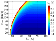
Since track conditions (head wind and adhesion) may vary during a single journey, the data from the remote sensors grid could be used within the developed model to estimate the journey’s duration and its feasibility for the particular track segment. The time frame map of the first 50 km of the proposed route from Figure 2 and the case of fully-loaded train is given in Figure 12. Normal passage time over this segment with this kind of load and with nominal 100% adhesion and 12 km/h head wind velocity, is 1.4 hour. Reduction of adhesion to around 70% and increase of head wind velocity to 40 km/h has negligible impact to the time increase. However, further reduction of adhesion or further increase of wind velocity significantly increases the segment passage time. White area in Figure 12 shows adhesion values and wind velocities corresponding to unfeasible driving missions for the particular train configuration, which could be used within the locomotive ‘telematic’ interface to alarm the driver of unfavourable driving conditions. Moreover, the data shown in Figure 12 may also be used to predict the possible problem of unscheduled stopping of the train due to insufficient powertrain capability to overcome the adverse weather-related track conditions. This might also prove to be highly useful in terms of managing train schedules by including an additional locomotive into the freight train in order to increase the traction capabilities and, thus, to reduce possible delays.
Train driving mission duration estimated for initial 50 km track segment under variable track conditions
Please note that the presented results have been obtained for the case of ideal availability of the remote sensor data in real time. Obviously, with the decrease of the availability of remote sensor data, the freight train control strategy adaptation would also deteriorate, thus resulting in the train driver model relying solely on the on-board train velocity measurements and slope information based on a-priori known rail track elevation profile. Thus, the presented adaptive control strategy would be reduced to the basic control strategy proposed in Cipek et al. [16] over the track segment characterised by low availability of real time remote sensor data. However, this type of scenario is beyond the scope of this work.
In this paper, the previously developed model of the battery-hybrid diesel-electric locomotive is extended with additional remote track condition data from the sensors network utilising 5G wireless communication technologies. These data are related to key two parameters defining the track conditions, i.e., the adhesion coefficient and the average head wind velocity, which, in turn, correspond to variable weather conditions. Those data are then used within the freight train model to predict its behaviour, and are also used to find optimal battery SoC controller parameters for different operating regimes, thus avoiding unnecessary deep discharging of the battery on-board the hybrid diesel-electric locomotive. The proposed approach has been extensively verified by means of comprehensive simulations.
The simulation model extended with variable track conditions has been able to identify the required adaptation of the driver behaviour (i.e., change of driving/braking regimes) under track adhesion and head wind variations. This has also resulted in increased time duration of the journey under the worsened track conditions (compared to the benchmark case with constant traction and head wind) in order to honour the related traction system limitations.
Worsened track conditions (i.e., lower adhesion and stronger head wind) also result in increased fuel consumption and deeper discharges of the battery energy storage system on board the hybrid diesel-electric locomotive due to sub-optimal operation of the power-train (i.e., diesel engine and the traction electrical drive). In particular, under reduced traction condition, the potential for freight train kinetic energy harvesting via the traction electrical drives is significantly reduced, whereas the increase in head wind generally results in increased power consumption.
The optimized SoC controller, utilising track condition information from the remote sensor network, can maintain the on-board battery SoC above the minimum recommended value (20% herein), which has not been the case with the fixed value SoC controller. Thus, the optimised controller is capable of preventing deep battery discharges associated with the battery useful life reduction, while simultaneously maintaining the fuel consumption at an acceptable level for the particular demanding driving scenario.
Final results also indicate that the model incorporating track condition data from remote sensors is also capable of predicting the driving mission duration over the track segment in question and of predicting possible unscheduled train halts due to adverse track conditions.
Future work may be directed towards investigation of availability of the wireless sensor network real-time data in terms of freight train control strategy adaptation and its general effect on the completion of driving mission and related safety issues, as well as more detailed investigation of the effectiveness of the proposed approach for different train configurations.
- ,
Transport Electrification: A Key Element for Energy System Transformation and Climate Stabilization ,Climatic Change , Vol. 123 (3-4),pp 651-664 , 2014, https://doi.org/https://doi.org/10.1007/s10584-013-0969-z - ,
Plug-in Vehicles and Renewable Energy Sources for Cost and Emission Reductions ,IEEE Transactions on Industrial Electronics , Vol. 58 (4),pp 1229-1238 , 2011, https://doi.org/https://doi.org/10.1109/TIE.2010.2047828 - ,
Determinants of Global CO2 Emissions Growth ,Applied Energy , Vol. 184 ,pp 1132-1141 , 2016, https://doi.org/https://doi.org/10.1016/j.apenergy.2016.06.142 - ,
Contribution of the Transport Sector to Climate Change Mitigation: Insights from a Global Passenger Transport Model Coupled with a Computable General Equilibrium Model ,Applied Energy , Vol. 211 ,pp 76-88 , 2018, https://doi.org/https://doi.org/10.1016/j.apenergy.2017.10.103 - ,
Environmental Impacts of Promoting New Public Transport Systems in Urban Mobility: A Case Study ,Journal of Sustainable Development of Energy, Water and Environment Systems , Vol. 5 (3),pp 377-395 , 2017, https://doi.org/https://doi.org/10.13044/j.sdewes.d5.0143 - ,
Sustainable Development Pathway for Intercity Passenger Transport: A Case Study of China ,Applied Energy , Vol. 254 (113632),pp 17 , 2019, https://doi.org/https://doi.org/10.1016/j.apenergy.2019.113632 - ,
A Review of the State-of-the-Art Technologies of Electric Vehicle, Its Impacts and Prospects ,Renewable and Sustainable Energy Reviews , Vol. 49 ,pp 365-385 , 2015, https://doi.org/https://doi.org/10.1016/j.rser.2015.04.130 - ,
Comparison and Evaluation of the Performance of Various Types of Neural Networks for Planning Issues Related to Optimal Management of Charging and Discharging Electric Cars in Intelligent Power Grids ,Emerging Science Journal , Vol. 1 (4),pp 201-207 , 2017, https://doi.org/https://doi.org/10.28991/ijse-01123 - Brussels, Belgium, https://ec.europa.eu/transport/facts-fundings/scoreboard/compare/energy-union-innovation/share-electrified-railway_en#2016
- ,
Novel Technologies and Strategies for Clean Transport Systems ,Applied Energy , Vol. 157 ,pp 563-566 , 2015, https://doi.org/https://doi.org/10.1016/j.apenergy.2015.09.051 - ,
Energy Storage Sizing Methodology for Mass-Transit Direct-Current Wayside Support: Application to French Railway Company Case Study ,Applied Energy , Vol. 230 ,pp 1673-1684 , 2018, https://doi.org/https://doi.org/10.1016/j.apenergy.2018.09.035 - ,
, Hybrid Locomotive, SUSTRAIL FP7 Project Deliverable 3.2.1, 265740 FP7 - THEME [SST.2010.5.2-2.] , 2014 - ,
Application of Flywheel Energy Storage for Heavy Haul Locomotives ,Applied Energy , Vol. 157 ,pp 607-618 , 2015, https://doi.org/https://doi.org/10.1016/j.apenergy.2015.02.082 - ,
Energy Storage Technologies and Hybrid Architectures for Specific Diesel Driven Rail Duty Cycles: Design and System Integration Aspects ,Applied Energy , Vol. 157 ,pp 619-629 , 2015, https://doi.org/https://doi.org/10.1016/j.apenergy.2015.05.015 - , , Ph.D. Thesis, 2009
- ,
Assessment of Battery-Hybrid Diesel-electric Locomotive Fuel Savings and Emission Reduction Potentials Based on a Realistic Mountainous Rail Route ,Energy , Vol. 173 ,pp 1154-1171 , 2019, https://doi.org/https://doi.org/10.1016/j.energy.2019.02.144 - ,
A Process-Based Model for Estimating the Well-To-Tank Cost of Gasoline and Diesel In China ,Applied Energy , Vol. 102 ,pp 718-725 , 2013, https://doi.org/https://doi.org/10.1016/j.apenergy.2012.08.022 - ,
A Survey on Future Railway Radio Communications Services: Challenges and Opportunities ,IEEE Communications Magazine , Vol. 53 (10),pp 62-68 , 2015, https://doi.org/https://doi.org/10.1109/MCOM.2015.7295465 - , , Proceedings of 13th Annual Conference on System of Systems Engineering (SoSE), 2018
- , , Proceedings of the 2009 International Symposium on Autonomous Decentralized Systems, 2009
- ,
Wireless Video Monitoring of the Megacities Transport Infrastructure ,Civil Engineering Journal , Vol. 5 (5),pp 1033-1040 , 2019, https://doi.org/https://doi.org/10.28991/cej-2019-03091309 - , , Proceedings of the 2018 IEEE Wireless Communications and Networking Conference (WCNC), 2018
- , , Adaptive Filtering and Change Detection, 2001
- , , Proceedings of the 11th European Conference on Antennas and Propagation (EUCAP), 2017
- ,
High-Speed Train Communications Standardization in 3GPP 5G NR ,IEEE Communications Standards Magazine , Vol. 2 (1),pp 44-52 , 2018, https://doi.org/https://doi.org/10.1109/MCOMSTD.2018.1700064 - , , Proceedings of 7th Transport Research Arena TRA 2018, 2018
- ,
Towards the Internet of Smart Trains: A Review on Industrial IoT-Connected Railways ,Sensors , Vol. 17 (1457),pp 44 , 2017, https://doi.org/https://doi.org/10.3390/s17061457 - ,
Internet of Things (IoT) in Industrial Engineering Education ,Acta Technica Corviniensis Bulletin of Engineering , Vol. 10 (2),pp 97-102 , 2017 - ,
5G Network-Based Internet of Things for Demand Response in Smart Grid: A Survey on Application Potential ,Applied Energy , Vol. 257 (113972),pp 15 , 2020, https://doi.org/https://doi.org/10.1016/j.apenergy.2019.113972 - ,
A Hierarchical Energy Management Strategy for Hybrid Energy Storage via Vehicle-To-Cloud Connectivity ,Applied Energy , Vol. 257 (113900),pp 9 , 2020, https://doi.org/https://doi.org/10.1016/j.apenergy.2019.113900 - ,
Dynamic Modeling and Experimental Investigation of Self-Powered Sensor Nodes for Freight Rail Transport ,Applied Energy , Vol. 257 (113969),pp 19 , 2020, https://doi.org/https://doi.org/10.1016/j.apenergy.2019.113969 - , 2016, https://metis-ii.5g-ppp.eu/wp-content/uploads/white_papers/5G-RAN-Architecture-and-Functional-Design.pdf
- , , Study on the Architecture of On-Board Radio Communication Equipment, Project Report No. ERA 2017 31 OP, 2018
- Stockholm, Sweden, 2016, https://www.ericsson.com/en/reports-and-papers/white-papers/cellular-networks-for-massive-iot--enabling-low-power-wide-area-applications
- ,
Narrow-Band Internet of Things: Implementations and Applications ,IEEE Internet of Things Journal , Vol. 4 (6),pp 2309-2314 , 2017, https://doi.org/https://doi.org/10.1109/JIOT.2017.2764475 - , , Impacts of Weather and Climate on American Railroading, 2006
- , , Proceedings of the 23rd Conference on IIPS / 87th American Meteorological Societys Annual Meeting, 2007
- ,
The Effects of Weather on Passenger Flow of Urban Rail Transit ,Civil Engineering Journal , Vol. 6 (1),pp 11-19 , 2020, https://doi.org/https://doi.org/10.28991/cej-2020-03091449 - ,
Weather Impact on Passenger Flow of Rail Transit Lines ,Civil Engineering Journal , Vol. 6 (2),pp 276-284 , 2020, https://doi.org/https://doi.org/10.28991/cej-2020-03091470 - Lyngby, Denmark, 2014, https://orbit.dtu.dk/ws/files/101319416/Management_of_low_adhesion_v12_Final.pdf
- ,
Gradient Modelling with Calibrated Train Performance Models ,WIT Transactions on the Built Environment , Vol. 127 ,pp 123-134 , 2012, https://doi.org/https://doi.org/10.2495/CR120111 - ,
Creep Forces in Simulations of Traction Vehicles Running on Adhesion Limit ,Wear , Vol. 258 (7-8),pp 992-1000 , 2005, https://doi.org/https://doi.org/10.1016/j.wear.2004.03.046 - , , Digital Proceedings of 3rd South East Europe (SEE) Sustainable Development of Energy Water and Environment Systems (SDEWES) Conference, 2018
- ,
Applicative Monitoring of Locomotive Diesel Engine Oil ,Fuels and Lubricants (Goriva i Maziva) , Vol. 43 (4),pp 291-309 , 2004 - , , Diesel-Electric Locomotives (in Croatian), 1985
- , http://www.gpsvisualizer.com/draw/
- , https://www.openrailwaymap.org/
- ,
Overview of Slip Control Methods Used in Locomotives ,Transactions on Electrical Engineering , Vol. 3 (2),pp 38-43 , 2014 - , , Proceedings of the ASME 2009 Dynamic Systems and Control Conference, 2009
- , , Ph.D. Thesis, 2005
- , , Digital Communications (5th ed.), 2008
- , , Keithley Instruments Inc., 2008
- , , Introduction to Signals and Systems, 1999
- , http://www.mathworks.com/products/communications.html