


Energy generated carbon emissions increased by approximately 2% between 2017 and 2018, arriving at more than 33 Gt CO2 in 2018. Additionally, approximately two-thirds of this growth can be attributed to the combustion of fossil fuels, particularly coal [1]. As a result, public concern regarding energy related global issues, particularly fossil fuel resource depletion and climate change is significantly rising. This has led several countries to look into different solutions to address these issues [2] and meet the Greenhouse Gas (GHG) emission reduction targets in the Parris Accord [3]. Climate change may be mitigated through advancing renewable energy sources, developing energy efficiency, and implementing carbon capture and storage technologies. However, these strategies are still limited by techno-economic and environmental bottlenecks [4].
As a renewable energy, biomass feedstock has garnered much attention in industry and research in the recent years since it can be converted into a wide array of bioenergy and bioproducts [5]. Co-firing biomass in existing coal-fired power plants is a promising approach to reduce GHG emissions. In fact, a co-firing ratio of 25% is reported to achieve near-zero emissions, and complete displacement of coal achieves negative emissions of more than 800 kg CO2 eq./MWh [4]. However, biomass inherently has a relatively higher moisture content than coal decreasing its lower heating value, which reduces the amount of energy that may be converted from it. Furthermore, most biomass residues have high alkali and ash content which can cause issues with molten ash deposition such as slagging or fouling, which can be corrosive to a boiler, when not properly managed. Although one of the advantages of biomass as an energy feedstock is its ability to be stored, its high volatile matter content when exposed to ambient moisture can lead to mass loss from vaporization during storage. Biomass pretreatment may also improve the transport efficiency of biomass by improving its bulk density. These issues may be addressed through pretreatment of the biomass [6].
Another critical configuration when implementing biomass co-firing is where biomass will be inserted in the power plants’ conversion process. The two most common co-firing configurations are direct and indirect co-firing. Direct co-firing involves burning a mixture of coal and biomass in a single common boiler. Although this requires minimal investment for the retrofitting of the plant, it can lead to corrosion in the equipment due to the unconventional fuel properties of the biomass-coal blend [7]. On the other hand, in indirect co-firing systems, biomass first undergoes gasification or pyrolysis for conversion into syngas and/or bio-oil, which is used as secondary fuel in direct co-firing systems. This set-up generates solid biochar residue which may be separated and applied to soil as fertilizer for further GHG reductions through carbon sequestration. Thus, indirect co-firing may result in negative emissions for the biomass fraction of the feedstock, even if total emissions still net positive due to the coal firing [3]. Nonetheless, the additional technology required for the separate gasifier makes implementing this configuration more expensive than direct co-firing, hence, it is less implemented in industry [8].
Negative Emission Technologies (NETs), such as direct air capture, augmented ocean disposal (i.e., ocean liming or fertilizer), bioenergy with carbon dioxide (CO2) capture and storage, and biochar application to soil, may become a critical approach to reduce CO2 levels in the atmosphere to safe levels. The last option has conventionally been used for soil conditioning but has become recognized as an effective strategy to mitigate climate change because it achieves the net removal of carbon from the atmosphere into the ground [9]. However, some researches contradict the benefits of biochar application. Some unintended consequents of this are the oversupply of nutrients, increased soil pH, impacts on germination and soil biological processes, binding and deactivation of agrochemicals (e.g., herbicides and nutrients) in the soil, and the release of toxic chemical contaminants in the biochar (e.g., heavy metals, polycylic aromatric hydrocarbons, and dioxins) [10]. These risks encourage the need to strategically match biochar sources, such as pyrolysis plants, to biochar sinks or agricultural lands and the associated soil conditions to minimize the potential negative effects of applying biochar to soil [9].
Given several complex challenges, proper management and design of the biomass supply chain networks, preferably supported by data-based decision-making tools such as optimization modelling, is crucial [11]. Several studies have proposed novel approaches to the optimal design biomass networks. Mohd Idris et al. [12] and Griffin et al. [13] developed multi-objective optimization models which minimized both costs and emissions for a biomass co-firing supply chain, while Pérez-Fortes et al. [14] formulated an optimization model which captures biomass quality to determine the optimal pretreatment scheme for biomass. However, the approach proposed by Pérez-Fortes et al. [14] is limited because it assumed strict constraints for quality requirements, when these limits are often violated in practice, while Mohd Idris et al. [12] and Griffin et al. [13] overlooked the consideration of feedstock properties despite its critical impact on system decisions and performance. San Juan et al. [15] and San Juan et al. [16] address this by developing a multi-objective optimization models that captures the changes in biomass properties as it moves along the supply chain and its impact on conversion yield and equipment damage. Most of these literatures which cover optimization modelling of co-firing supply chain focus only on direct co-firing despite the trade-offs between the two co-firing schemes [17]. San Juan et al. [15] and Aviso et al. [3] are works which address these gaps in literature by developing optimization models which consider the selection between direct and indirect co-firing integrated with biochar-based carbon sequestration. However, these two studies assume simplistic and deterministic conditions.
Biochar carbon management networks are natural extensions of upstream biomass-based energy systems [18]. Nonetheless, previous studies have modelled them as stand-alone systems. Tan [9] was the first to consider the optimal synthesis of biochar-based carbon management networks in a mixed integer linear programming model which identified the optimal allocation of biochar with varying contaminant levels to a set of biochar sinks with predefined storage capacities and contaminant level limits over a multiple period planning horizon. This initial model proposed by Tan [9] was extended by Belmonte et al. [10] and Belmonte et al. [19] using a two-stage and a bi-objective optimization model, respectively. These two studies optimized economic and environmental objectives, specifically minimizing costs and maximizing CO2 sequestration. Belmonte et al. [19] improved on previous approaches by considering the dependence of carbon sequestration on the interactions between the biochar and biochar sinks because the success of these systems does not only rely on feedstock materials and processing conditions, but are also influenced by the type and quality of the soil to which the biochar is applied to. Nonetheless, the need to capture upstream and downstream activities in a holistic analysis to capture interactions between them were not yet explored in these studies.
Even though biomass co-firing systems have been found to generate both economic and environmental benefits, a series of issues influenced by internal and external uncertainties also come with it. These uncertainties are traditionally overlooked even though they could render optimal solutions infeasible or significantly suboptimal. With this, the proper construction and management of a biomass co-firing network such that it is invulnerable to uncertainties becomes an important challenge to overcome. Biomass co-firing network design projects entail both investment and operational decisions including retrofits on existing handling systems in coal-fired power plants, biomass and coal purchase and transport, installation of biomass pretreatment technology or facilities, and energy production planning. Investment decisions are usually expensive and challenging to reverse, and have long-term and significant influence on the networks overall economic and environmental performance. Biomass properties are inherently plagued with uncertainties significantly influenced by external factors, such as climate, weather, and cultivation and harvesting approaches, the effect of these separately and their interactions are difficult to predict. Furthermore, biomass properties are endogenous in nature, wherein their properties are uncertain prior to conversion, and will be resolved depending on the co-firing configuration chosen and the conversion yield. However, only uncertainties in supply, demand, and prices are commonly considered in biomass co-firing supply chain network design models [20]. Given the impact of realizations of uncertainties on a system, several researchers have been spurred to incorporate uncertainty through stochastic parameters in designing biomass networks. Only Castillo-Villar et al. [21] considered biomass quality as an uncertainty in a biomass supply network design problem, but the impact of biomass quality was modelled only as additional costs incurred from pretreatment. San Juan and Sy [22] proposed a robust optimization model considering only the lower heating value of biomass as the uncertain parameter. However, there are several aspects of biomass quality that have significant impact on supply chain decisions, such as moisture content, ash content, and bulk density.
This study develops a novel robust optimization model for the optimal synthesis and planning of a multi-echelon network composed of biomass and coal allocation to pretreatment facilities for co-firing in existing coal power plants integrated with biochar allocation networks for carbon sequestration. The model takes into consideration power demand, biomass and coal supply, plant capacities, and biochar application limits to simultaneously minimize costs and emissions while subject to uncertain biomass properties. The proposed robust approach may be used to identify a range of solutions depending on the risk appetite of the decision maker. Each solution maximizes the robustness index, which is a measure of how much uncertainty the solution will be able to tolerate before it becomes infeasible, whilst ensuring that economic and environmental targets are satisfied. This feature reduces inherent weakness of the traditional robust optimization of producing solutions that are overly conservative. Furthermore, the robust approach preserves the computational tractability of the deterministic problem, unlike when using stochastic optimization which is typically computationally expensive [23]. The resulting formulation may easily be solved by commercially available solvers.
The rest of the paper is organized as follows. Section 2 provides the formal problem statement, while Section 3 discusses the development of the Multi-objective Target-oriented Robust Optimization (MOTORO) model. Then, a biomass co-firing network case study is discussed and solved to demonstrate the capabilities of the proposed model in Section 4, a comparison between the deterministic and robust solution is presented to highlight the advantage of utilizing the MOTORO methodology. Finally, Section 5 gives the conclusions and recommendations for future work.
The formal problem statement can be stated as follows:
The biomass co-firing network has biomass waste sources (i), coal sources (j), biomass pretreatment facilities (k), existing coal power plants (l), and biochar sinks (n), wherein the solid biochar by-product produced from coal power plants configured for indirect co-firing may be brought for permanent carbon sequestration, studied across a planning horizon of periods (t);
Each biomass source has a maximum available supply of biomass each period with corresponding bulk density, moisture content, and ash content, which may be purchased at a certain price. However, the moisture and ash contents of the biomass experiences variabilities, represented by a range of percentages where the upper and lower limits reflect the most pessimistic and optimistic scenarios, respectively;
Each coal source has a maximum availability supply of coal each period that may be purchased at a certain price. The coal has constant bulk density, lower heating value, and moisture content and ash contents;
Raw biomass may be processed in pretreatment facilities to improve their moisture and ash contents by a certain percentage and their bulk densities specific to each facility. Each pretreatment facility can only process a certain amount of biomass each period with associated fixed and variable costs, but processing capacities may be increased for a certain fixed and proportional costs. Additionally, treated biomass may be kept in inventory for future periods limited by each facility’s storage capacity with associated costs, but capacity may also be expanded with corresponding expansion costs. Aside from costs, processing biomass in pretreatment facilities generate GHG emissions;
Each coal power plant may be retrofitted to implement f co-firing schemes with a retrofitting cost. Each coal power plant and co-firing scheme have corresponding upper and lower coal displacement limits, which sets an allowable range for how much coal can be safely displaced by biomass. If co-firing is implemented in a power plant, a mix of raw and treated biomass and coal may be converted into energy to satisfy energy demand each period, limited by a certain processing capacity that may be increased through capacity expansion. Nonetheless, there are corresponding fixed and variable costs to process biomass and coal feedstock, as well as to expand the capacities of each coal power plant, and GHG emissions are generated through burning coal. If direct co-firing is chosen, the equipment in the power plants may experience damage from the unconventional properties of the feedstock mix when it violated allowable limits for ash and moisture contents, which decreases the conversion efficiency of the power plants. Each power plant has a certain efficiency threshold. If the plant’s efficiency falls below this threshold, it must be shut down until repair or maintenance is performed, which also has corresponding costs. However, when indirect co-firing is implemented, a fraction of the biomass feedstock processed by the plant will be converted into biochar, which has a particular bulk density. Each plant generates biochar with different concentrations of c contaminants;
Each biochar sink has a sequestration factor, maximum biochar capacity, and maximum tolerance for contaminant c;
The distances between each potential source-destination pair, together with the corresponding cost and carbon footprint from transportation of biomass, coal, and biochar proportional to each unit of distance travelled.
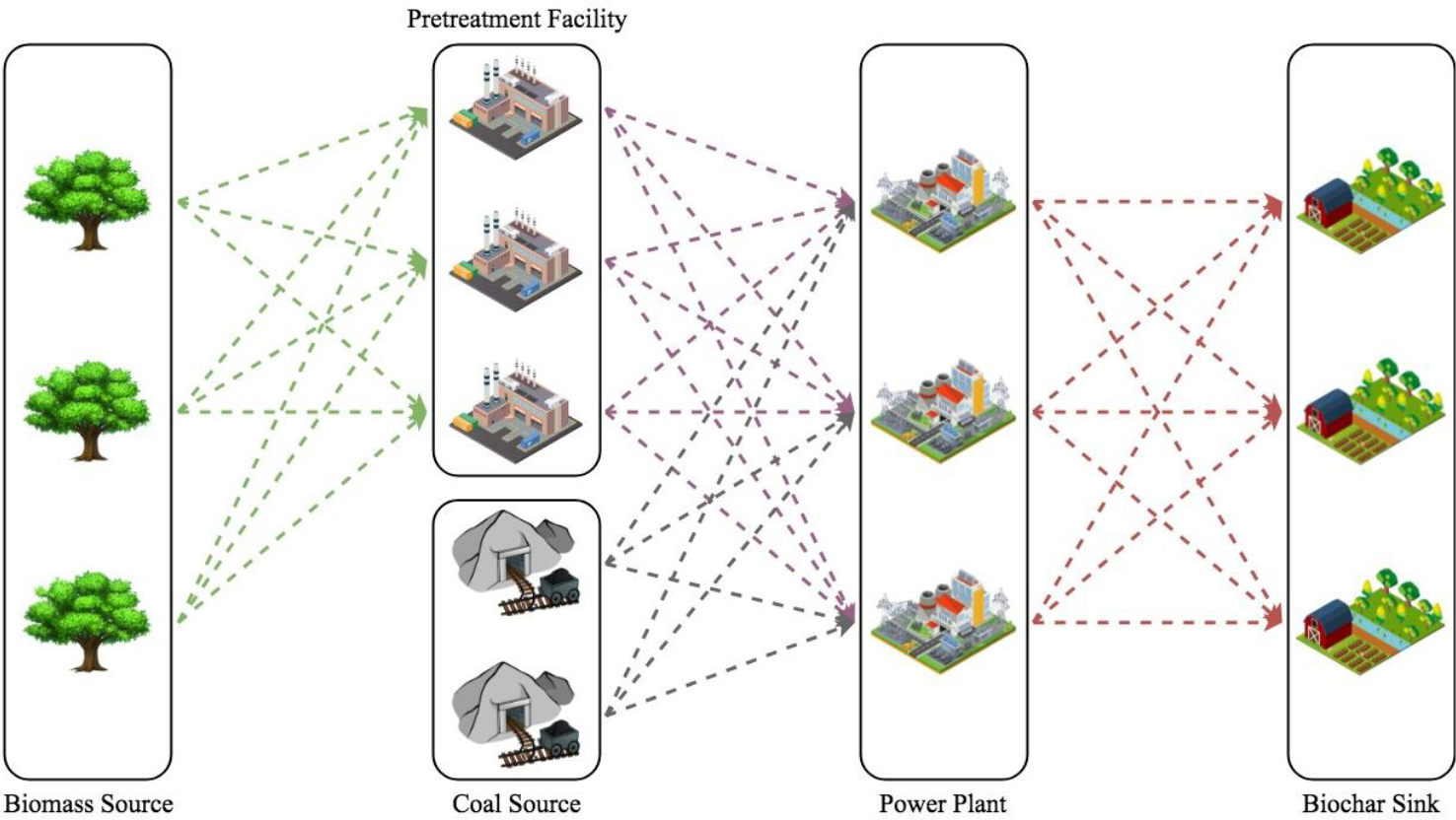
The problem may be visualized as a superstructure shown in Figure 1. The objective is to determine the optimal allocation of raw biomass from sources to pretreatment facilities and coal power plants, pretreated biomass from pretreatment facilities to coal power plants, coal from sources to coal power plants, and biochar from coal power plants to biochar sinks, to identify which existing coal power plants must be retrofitted and the co-firing scheme to be implemented, which pretreatment facilities and coal power plants should be operating each period, as well as the schedule for implementing the co-firing option to maximize robustness index θ of the resulting network design influenced by variations in biomass quality while simultaneously satisfying cost and environmental impact targets. The solution should also indicate whether biomass should be kept in inventory in a pretreatment facility each period, whether the capacities of the pretreatment facilities and coal power plants should be increased, and whether the equipment in the coal power plants need to undergo maintenance or repair.
Network superstructure
This section presents the model formulation for the biomass co-firing network system described beginning with a definition of the relevant variables and parameters, followed by the development of the deterministic model, which does not yet account for any uncertainties. The basic optimization model is revised to account for uncertainties in the biomass’ moisture and ash contents through the application of the MOTORO approach.
The basic optimization model for the biomass co-firing network understudy is shown in eq. (1-60) wherein the overall objectives of the system are to minimize economic costs and environmental emissions. The total economic cost is expressed in eq. (1) as the sum of costs incurred from operating the pretreatment facilities and power plants, holding inventory, expanding storage, pretreatment, and coal power plant capacities, purchasing feedstock, transporting biomass, coal, and biochar, applying biochar to soil, and repairing or performing maintenance on power plant equipment each period, incurring unmet demand, as well as the costs to retrofit existing coal power plants, shown individually in eq. (2-11). Transportation costs are proportional to the total distance travelled and the average transportation cost per unit distance:
(1)
(2)
(3)
(4)
(5)
(6)
(7)
(8)
(9)
(10)
(11)
The model also aims to minimize the net carbon emissions of the biomass co-firing network expressed in eq. (12) as the sum of emissions from transporting biomass, coal and biochar, burning coal for power generation, and pretreating biomass across all periods in the planning horizon shown in eq. (13-15). Similarly, total emissions from transporting feedstock is based on emissions per unit distance and total distanced travelled:
(12)
(13)
(14)
(15)
(16)
The net emissions contributed by the network may be reduced through carbon sequestration from utilizing biochar as soil amendment expressed in eq. (16). Eq. (17) computes for the demand for power satisfied each period. The amount of energy produced each period is computed for by multiplying the conversion efficiency of each coal power plant for a particular period, lower heating value of the mixed fuel being handled, and the total amount of feedstock processed by the coal power plant. The total amount of biomass fed into the handling equipment of the power plant is dependent on the biochar yield of the co-firing scheme implemented and the amount of biomass received by the coal power plant. If direct co-firing scheme is implemented, biochar yield is equal to zero, allowing the coal power plant to process all of the biomass it received. On the other hand, if indirect co-firing scheme is chosen, a fraction of the biomass would have been converted to biochar and would not undergo conversion to electricity. The formulation in eq. (17) makes demand satisfaction a soft constraint and allows for the possibility for unmet demand and overshooting the demand. However, the amount of feedstock processed by the coal power plant must be less than or equal the processing capacity as enforced in eq. (18). Eq. (19) and eq. (20) limits the amount of biomass and coal that can be purchased and transported from each source location to the source’s available supply each period:
(17)
(18)
(19)
(20)
Eq. (21) ensures that a specific co-firing scheme may only be used if the power plant has been retrofitted for that particular co-firing scheme, while eq. (22) defines the co-firing schemes as mutually exclusive options. Eq. (23) set upper and lower coal displacement limits to the biomass and coal blends that will be used in each power plant and period depending on the co-firing scheme implemented:
(21)
(22)
(23)
The amount of biomass brought to the pre-treatment facilities should be less than or equal to the processing capacity of each facility, as shown in eq. (24). The weight of the biomass received by a pre-treatment facility in each period after undergoing pre-treatment processes is given in eq. (25), which is given by adding the pure biomass weight and the remaining moisture and ash content left after completing treatment. The inventory of biomass kept in the pre-treatment facilities is defined in eq. (26) as equal to the amount of biomass carried over from the previous period and received from sources and pre-treatment facilities, less the biomass sent to the power plants in the current period. Eq. (27) makes sure that the amount of biomass held each period is restricted by the facility’s storage capacity:
(24)
(25)
(26)
(27)
The capacities of the pre-treatment facilities and the coal power plants may be expanded. Eq. (28-30) show that the processing and storage capacities assigned to each facility are dependent on the capacity expansion performed in the previous period. Binary variables for capacity expansions are switched on in eq. (31-33):
(28)
(29)
(30)
(31)
(32)
(33)
Eq. (34) computes for the moisture content of the biomass that has just completed pre-treatment and mixed with the existing biomass in stock. The improved moisture content is computed for by dividing the remaining moisture in biomass by weight and moisture in the biomass kept in stock with the total biomass in each pre-treatment facility. Eq. (35) defined the average moisture content of all the biomass received by a coal power plant in each period. Lastly, eq. (36) computes for the moisture content of the mixed feedstock processed by the coal power plant handling equipment. The ash content of the feedstock as it moves through the network is similarly computed for in eq. (37-39):
(34)
(35)
(36)
(37)
(38)
(39)
Eq. (40) determines the lower heating value of the biomass in each coal power plant. This equation is adapted from the research of Hernández et al. [24], which estimates the lower heating value by subtracting the latent heat of vaporization of water from the higher heating value. The computation for the average lower heating value of the feedstock of a plant considering the biomass and coal blend is given in eq. (41):
(40)
(41)
The conversion equipment in all of the coal power plants begin with conversion efficiencies of 100%. The percentage conversion efficiency in each power plant is a function of the excess and lacking moisture content of the feedstock, excess ash content, and the total amount of feedstock processed by the plant, as these values increase, the efficiency will decrease, and may be increased by repair or maintenance as shown in eq. (42). Eq. (43) describes accumulated excess moisture content to be equal to the excess moisture content for the current period, which is the maximum between zero and the difference between the actual moisture content of the feedstock and the upper limit, and the accumulated excess moisture content of the previous period, while eq. (44) defines accumulated shortage in moisture. Similarly, eq. (45) and eq. (46) computes for the accumulated excess and shortage in ash content. With this approach, there will be no amount stored if the difference returned is negative. Lastly, eq. (47) sums up the biomass and coal processed in a coal power plant each period to get the total feedstock handled by the equipment and adds this to the accumulated values from previous. Furthermore, the computations for quality violations in eq. (43-47) are dependent on the risk for equipment damage of the specific co-firing scheme implemented in the power plant:
(42)
(43)
(44)
(45)
(46)
(47)
Eq. (48) activates switches for repair or maintenance and limits the percent effectiveness of maintenance to a maximum of one. Eq. (49) makes sure that when the efficiency of the coal power plant falls below the plant’s efficiency threshold, the coal power plant cannot be allowed to operate. On the other hand, when the conversion efficiency of the coal power plant is above the threshold, the coal power plant can choose whether or not to operate for that period:
(48)
(49)
The amount of biochar that may transported from coal power plants is shown in eq. (50) is limited by the product between the amount of biomass processed and the fraction biochar yield of the co-firing scheme selected. Eq. (51) limits the amount of biochar allocated to each sink by the storage capacity of the sink, while eq. (52) ensures that the contaminant levels of the biochar allocated to each sink does not exceed the allowable contaminant levels, which is given by the decision maker’s tolerance for soil contaminants and the limits for each contaminant type:
(50)
(51)
(52)
Eq. (53-57) compute for the number of trips needed to transport biomass, coal, and biochar from their respective sources and destinations based on the weight and volume capacities of the transport vehicles:
(53)
(54)
(55)
(56)
(57)
Lastly, non-negativity, binary, and integer constraints are imposed on the relevant variables in eq. (58-60):
(58)
(59)
(60)
However, there is a need to consider uncertainties that may be realized from biomass quality variability, particularly its moisture and ash contents, when designing and planning biomass co-firing networks. This uncertainty can significantly impact the economic and environmental sustainability and feasibility of the design, thus, the implemented setup should remain feasible despite realizing the highest potential degree of uncertainty. The basic optimization model is modified to account for uncertainties in moisture and ash contents denoted by and , respectively. The revised formulation considering these uncertainties is given by eq. (60-65) replacing eq. (25), eq. (34), eq. (35), eq. (37), and eq. (38):
(61)
(62)
(63)
(64)
(65)
The sources of uncertainty, particularly the uncertain biomass moisture () and ash content (), are incorporated through the Target-Oriented Robust Optimization (TORO) approach proposed by Ng and Sy [23], which is extended to capture several objectives through the MOTORO approach. MOTORO facilitates optimal network design and planning through the achievement of targets derived under uncertainty. Appropriate values for the decision variables should be identified so that the system constraints remain feasible for the largest range of the uncertain parameters as possible. These sources of uncertainty could then be defined as perturbations in the biomass moisture () and ash content () from their nominal values and and as shown in eq. (66) and eq. (67):
(66)
(67)
(68)
Eq. (68) shows that the robustness index quantifies the degree of uncertainties in the given parameters. For instance, the largest perturbation occurs when and , for all i = 1, …, I and t = 1, …, T. This is associated with a robustness index of θ = 1.0. This also assumes that under the most favorable case, and would be at the minimum and equal to the nominal values, which are associated with a robustness index of θ = 0.0 since no perturbation from the nominal values can be accommodated. This follows because moisture and ash content indirectly impact the energy conversion yield, equipment efficiency, and pretreatment costs and emissions. These perturbations are parameterized by the robustness index .
The concept of the MOTORO approach is based on the integration of the robust optimization framework and target-oriented decision making. Target-oriented decision making is reflected in the model by translating the original objective of costs and emissions minimization into system targets that consider the different scenarios that result from biomass quality uncertainty. This procedure allows the decision maker to select among non-dominated solutions based on how much risk or uncertainty they are willing to tolerate. Eq. (69) shows the modified objective function, which now maximizes the robustness index (), which is the degree of uncertainty that can be tolerated by a solution before it becomes infeasible. A higher value of θ implies a larger degree of perturbation for the biomass properties, thus, a more risk-averse decision maker would prefer a higher θ because it is more robust. This replaces and is subject to the previously shown objective functions, which are translated into costs () and emissions () targets shown in eq. (70) and eq. (71), and the other function constraints discussed earlier. The bisection search algorithm is used to maximize θ:
(69)
(70)
(71)
Targets are set using the equations shown in eq. (72) and eq. (73), which can be used by decision makers as a guide when setting their targets. Setting targets that are too optimistic results in the risk of missing these targets, on the other hand, establishing too conservative targets limits the results of the model, which could lead to significant opportunity losses for the network owners:
(72)
(73)
Eq. (72) and eq. (73) can be used to identify a range of targets through the parameter for both costs and emissions. In the two equations, and reflect the costs and emissions under the most optimistic conditions where , while and represent the most pessimistic conditions where . The level is the parameterized index for perturbations of the uncertain parameters, higher values imply that a decision maker is conservative, while lower values are chosen by decision makers with more risk-appetite. In this system, a more risk-averse decision maker would assume worse or higher values for moisture and ash content in biomass, while a less risk-averse decision maker would assume the opposite. The maximum robustness index that minimizes both costs and emissions at different cost and emissions targets is determined with different levels of using the bisection method algorithm shown in Table A1.
Computational experiments were carried out using IBM ILOG CPLEX Optimization Studio in MATLAB on a MacBook Pro with a 3.1 GHz Intel Core i5 processor and 8 GB 2133 MHz LPDDR3 RAM. The CPLEX solver allows MATLAB to solve linear optimization problems through a simplex algorithm. Nonlinear equations were linearized to facilitate this, and a decomposition algorithm was also utilized. A hypothetical case study is used to validate the proposed model. The system considered is composed of six biomass sources, four coal sources, three pretreatment facilities, four existing coal power plants, three biochar sinks across a five-year planning horizon. The input parameters used in the validation of the proposed model were adopted and modified from several existing studies, particularly co-firing costs parameters from Griffin et al. [13], while biochar application parameters were sourced from Tan [9].
Table 1 shows the costs associated with retrofitting, operating, expanding the capacity, and performing maintenance on the existing power plants. Variable costs are proportional to the amount of biomass and coal processed by the power plant. Meanwhile, it costs USD 1.2 to burn each kilogram of feedstock. Similarly, the costs associated with operating the pretreatment facilities and their corresponding storage facilities are shown in Table 2. Table 2 also details the fixed and variable costs incurred by the system to expand the processing and storage capacities of the pretreatment facilities. Transportation costs are assumed to be USD 26.16 per kilometer travelled. The costs to purchase each kilogram of biomass and coal from their respective sources are USD 0.0149 and USD 0.06, respectively. Applying biochar to soil as amendment will also incur the system costs, particularly USD 0.0149 per kilogram of biochar applied.
Power plant costs
| Power plant | Retrofitting co-firing | Operating | Expansion | Maintenance | |||
|---|---|---|---|---|---|---|---|
| Direct [USD] | Indirect [USD] | Fixed [USD] | Fixed [USD] | Variable [USD/kg] | Fixed [USD] | Variable [USD/kg] | |
| 1 | 22,000 | 58,000 | 2,500 | 500 | 15 | 750 | 75 |
| 2 | 23,000 | 69,000 | 5,600 | 400 | 20 | 600 | 50 |
| 3 | 32,500 | 47,500 | 4,450 | 450 | 10 | 800 | 60 |
| 4 | 22,500 | 67,200 | 3,500 | 400 | 15 | 675 | 25 |
Pretreatment facility costs
| Pretreatment facility | Processing | Processing expansion | Storage | Storage expansion | ||||
| Fixed [USD] | Variable [USD/kg] | Fixed [USD] | Variable [USD/kg] | Fixed [USD] | Variable [USD/kg] | Fixed [USD] | Variable [USD/kg] | |
| 1 | 200 | 0.09 | 400 | 20 | 120 | 0.02 | 400 | 20 |
| 2 | 300 | 0.05 | 450 | 10 | 105 | 0.01 | 450 | 10 |
| 3 | 500 | 0.04 | 500 | 15 | 100 | 0.05 | 500 | 15 |
The carbon emissions from treating each kilogram of biomass in each pretreatment facility are shown in Table 3. Additionally, burning coal to produce energy also results in carbon being emitted into the atmosphere. The amount of carbon released from the combustion of each kilogram of carbon is 5.86 kg CO2. Transportation emissions are assumed to be 0.0005 kg CO2 per distance travelled. The emissions parameters were adapted from the study of Mohd Idris et al. [12].
Biomass pretreatment emissions
| Pretreatment facility | Emissions [kg CO2/kg] |
| 1 (torrefaction) | 0.01 |
| 2 (pelletization) | 0.03 |
| 3 (torrefaction + pelletization) | 0.04 |
Demand is assumed to differ every period, the demand experienced by the system is shown in Table 4, while biomass and coal supply is only assumed to vary between each source. The initial capacities of the coal power plants and pretreatment facilities were arbitrarily set to 35,000 kg, while the storage facilities within the pretreatment facilities had initial capacities of 10,000 kg. The bulk densities, moisture and ash contents of raw biomass from each source are detailed in Table 5. Two columns are given for both biomass moisture and ash contents to provide the range across which the uncertain parameters are assumed to vary along. The values adopted for the biomass’ higher heating value is 16.71 MJ/kg, hydrogen content is 6.5%, nitrogen content equals to 1.7%, and oxygen content is 47.5%. Biomass property values were adopted from the researches of Kargbo et al. [25] and Liu et al. [26]. For the deterministic and base run model validation, the median values were used for moisture and ash content. The bulk density, lower heating value, ash content, and moisture content of coal are assumed to be 793 kg/m3, 22.73 MJ/kg, 7.5%, and 9.05%, respectively [27].
Demand and supply parameters
| Period [year] | 1 | 2 | 3 | 4 | 5 | |
| Demand [MJ] | 500,000 | 600,000 | 550,000 | 600,000 | 540,000 | |
| Biomass source | 1 | 2 | 3 | 4 | 5 | 6 |
| Supply [kg] | 4,500 | 4,500 | 5,700 | 5,500 | 6,000 | 5,750 |
| Coal source | 1 | 2 | 3 | 4 | ||
| Supply [kg] | 20,000 | 20,000 | 20,000 | 20,000 |
Biomass quality parameters
| Biomass source | Moisture content [% mass] | Ash content [% mass] | Bulk density [kg/m3] | ||
| 1 | 7 | 21 | 9 | 18 | 50 |
| 2 | 9 | 19 | 5 | 20 | 60 |
| 3 | 11 | 23 | 10 | 23 | 20 |
| 4 | 7 | 18 | 7 | 15 | 35 |
| 5 | 9 | 20 | 10 | 18 | 80 |
| 6 | 8 | 25 | 8 | 17 | 55 |
Because each pretreatment facility is assumed to perform a different type of pretreatment process, different efficiencies for ash content and moisture content improvement efficiency are assigned to each pretreatment facility. In the same way, the bulk density of treated biomass differs between pretreatment facilities. These parameters are shown in Table 6. Parameters for moisture content and bulk density improvement were adapted and modified from Pérez-Fortes et al. [14], which shows a range of pretreatment technologies including torrefaction, pelletization, pyrolysis, and their combinations, while ash content improvements were assumed. It is assumed that the system starts with no biomass in inventory.
Biomass pretreatment parameters
| Pretreatment facility | Moisture content [% improvement] | Ash content [% improvement] | Bulk density [kg/m3] |
| 1 (torrefaction) | 80 | 25 | 230 |
| 2 (pelletization) | 10 | 35 | 575 |
| 3 (torrefaction + pelletization) | 90 | 20 | 800 |
Upper and lower coal displacement limits are enforced in each retrofitted coal power plant depending on the co-firing scheme it has been modified for as presented in Table 7. In this model, the upper displacement limit is higher for indirect co-firing systems because biomass is separately processed from coal. The limits for the moisture and ash contents of the mixed fuel processed in each coal power plant is also given in Table 8. The risk of damage in the equipment from processing biomass is influenced by the co-firing scheme implemented. It is assumed that if indirect co-firing scheme is chosen, no damage occurs due to moisture content and ash content properties, while full risk is experienced when direct co-firing is chosen. The efficiency threshold for each coal power plant represents the lower bound of the conversion efficiency. This forces a coal power plant to close down unless repairs or maintenance on the equipment is performed. The efficiency threshold is assumed to be 0.3 or 30%, the same for all power plants. The biochar yield is dependent on the co-firing scheme implemented. When direct co-firing scheme is implemented, no biochar will be produced. On the other hand, when indirect co-firing is chosen, it is assumed that 20% of the biomass fraction of the feedstock is transformed into biochar.
Coal displacement limits and quality tolerances parameters
| Co-firing scheme | Displacement limit | Feedstock property | Property/Quality limit [% mass] | ||
| Lower | Upper | Lower | Upper | ||
| Direct | 0 | 0.2 | Ash | 3.3 | 8 |
| Indirect | 0 | 0.5 | Moisture content | 2.2 | 12 |
Biochar properties
| Power plant | Biochar quality [mg PAH/kg] | Biochar quality [mg Zn/kg] | Biochar quality [mg Pb/kg] |
| 1 | 10 | 50 | 2 |
| 2 | 2 | 10 | 1 |
| 3 | 1 | 5 | 0.5 |
| 4 | 8 | 20 | 4 |
Biochar sink properties
| Biochar sink | Storage capacity [kg] | Sequestration factor [kg CO2/kg] | Biochar quality limit | ||
| [mg PAH/kg] | [mg Zn/kg] | [mg Pb/kg] | |||
| 1 | 1,800 | 5.2 | 250 | 200 | 40 |
| 2 | 1,800 | 5.0 | 100 | 125 | 30 |
| 3 | 5,400 | 5.5 | 50 | 500 | 120 |
Depending on the processes undergone, biochar may have different concentration of contaminants. Thus, the contaminant levels in biochar differs based on the power plant from which it was produced. The contaminants considered in the model validation are Polycyclic Aromatic Hydrocarbons (PAH) and heavy metals, zinc (Zn) and lead (Pb). The presence of these contaminants in biochar utilized as soil amendment for crop plant cultures can pose a potential disadvantage from ecotoxicity risk [10]. These values are shown in Table 8. The allowable soil contaminant factor (ψ) represents the willingness of the decision maker to contaminate soil properties with biochar contaminants and can assume values varying between 0 to 1. For the purpose of the validation, this is assumed to be equal to 1. The total biochar storage capacity of each sink is shown in Table 9. Similarly, Table 9 also presents the sequestration factor of biochar applied in each sink and the maximum allowable concentration of each contaminant in each biochar sink. Lastly, the bulk density of biochar is assumed to be 200 kg/m3.
Table 10 and Table 11 show the distances in kilometres between biomass sources to pretreatment facilities, pretreatment facilities to coal power plants, biomass sources to coal power plants, coal sources to coal power plants, and coal power plants to biochar sinks. Additionally, the weight and volume capacities are assumed to be 13,500 kg and 55 m3, respectively.
Distances between biomass sources, pretreatment facilities, and power plants [km]
| Biomass source | Pretreatment facility | Power plant | Pretreatment facility | Power plant | ||||||||
| 1 | 2 | 3 | 1 | 2 | 3 | 4 | 1 | 2 | 3 | 4 | ||
| 1 | 30 | 40 | 35 | 40 | 50 | 45 | 40 | 1 | 15 | 15 | 20 | 15 |
| 2 | 25 | 40 | 30 | 25 | 50 | 40 | 45 | 2 | 20 | 20 | 20 | 20 |
| 3 | 15 | 45 | 35 | 25 | 55 | 45 | 35 | 3 | 20 | 18 | 17 | 15 |
| 4 | 30 | 20 | 25 | 40 | 20 | 35 | 40 | |||||
| 5 | 15 | 20 | 15 | 25 | 30 | 25 | 35 | |||||
| 6 | 35 | 25 | 35 | 45 | 35 | 45 | 45 | |||||
Distances between coal sources, power plants, and biochar sinks [km]
| Coal sources | Power plant | Power plant | Biochar sink | |||||
| 1 | 2 | 3 | 4 | 1 | 2 | 3 | ||
| 1 | 30 | 35 | 25 | 35 | 1 | 15 | 10 | 15 |
| 2 | 30 | 25 | 20 | 30 | 2 | 10 | 15 | 15 |
| 3 | 30 | 30 | 30 | 30 | 3 | 15 | 15 | 10 |
| 4 | 25 | 35 | 30 | 30 | 4 | 10 | 10 | 15 |
The relationship between conversion equipment efficiency, feedstock property violations and total feedstock processed is modelled with an arbitrary function. For the model validation, an exponential decay function is chosen, the conversion efficiency of the equipment is equal to a certain constant raised to the feedstock quality violations and volume of feedstock processed as shown in eq. (74):
(74)
An exponential function with a base that is greater than or equal to 1 will return decreasing values as the exponent variables increase. Efficiency will begin at 1 when the exponent is 0 or when no feedstock property violations have been made and/or no feedstock has been handled by the power plant yet. The efficiency value will then decrease, approaching 0 as the exponent increases. The constant dictates the rate of decrease per unit increase in the exponent variables. The higher the constant the faster the rate of decrease will be. For the model validation, the constant used was e, which has an approximate value of 2.7183.
The optimization of the deterministic model returns a total system cost of USD 1,535,762.55 and emissions of 568,500.37 kg CO2, which were both minimized. Majority of the costs may be attributed to power plant retrofitting costs because all plants were retrofitted for indirect co-firing. Despite biomass displacing, coal for energy production through the implementation of co-firing in all of the coal power plants, majority of the environmental emissions is contributed by coal combustion for energy generation. Nonetheless, significant reductions in emissions is achieved through biochar-based carbon sequestration, which achieved 170,629 kg CO2 carbon sequestration.
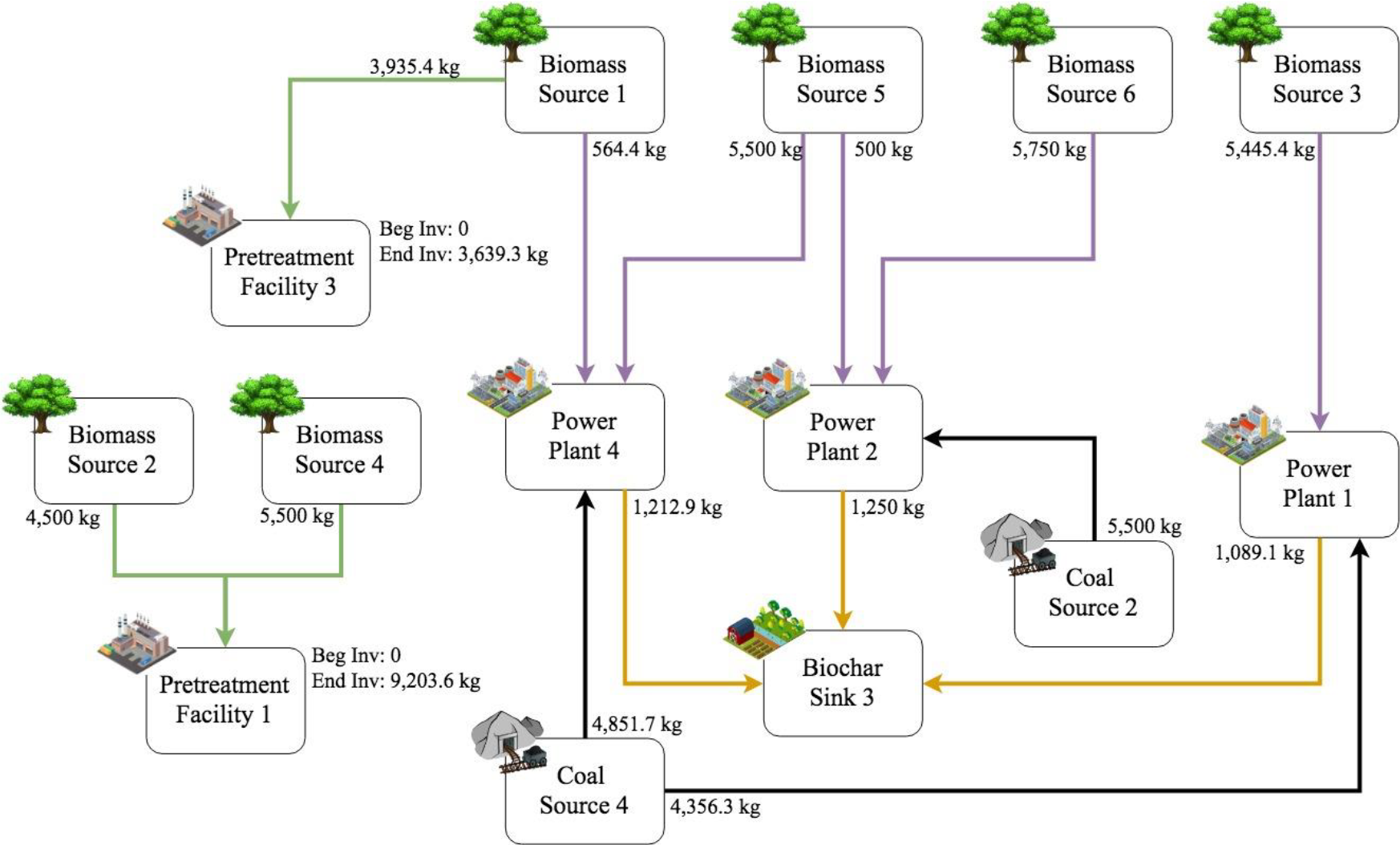
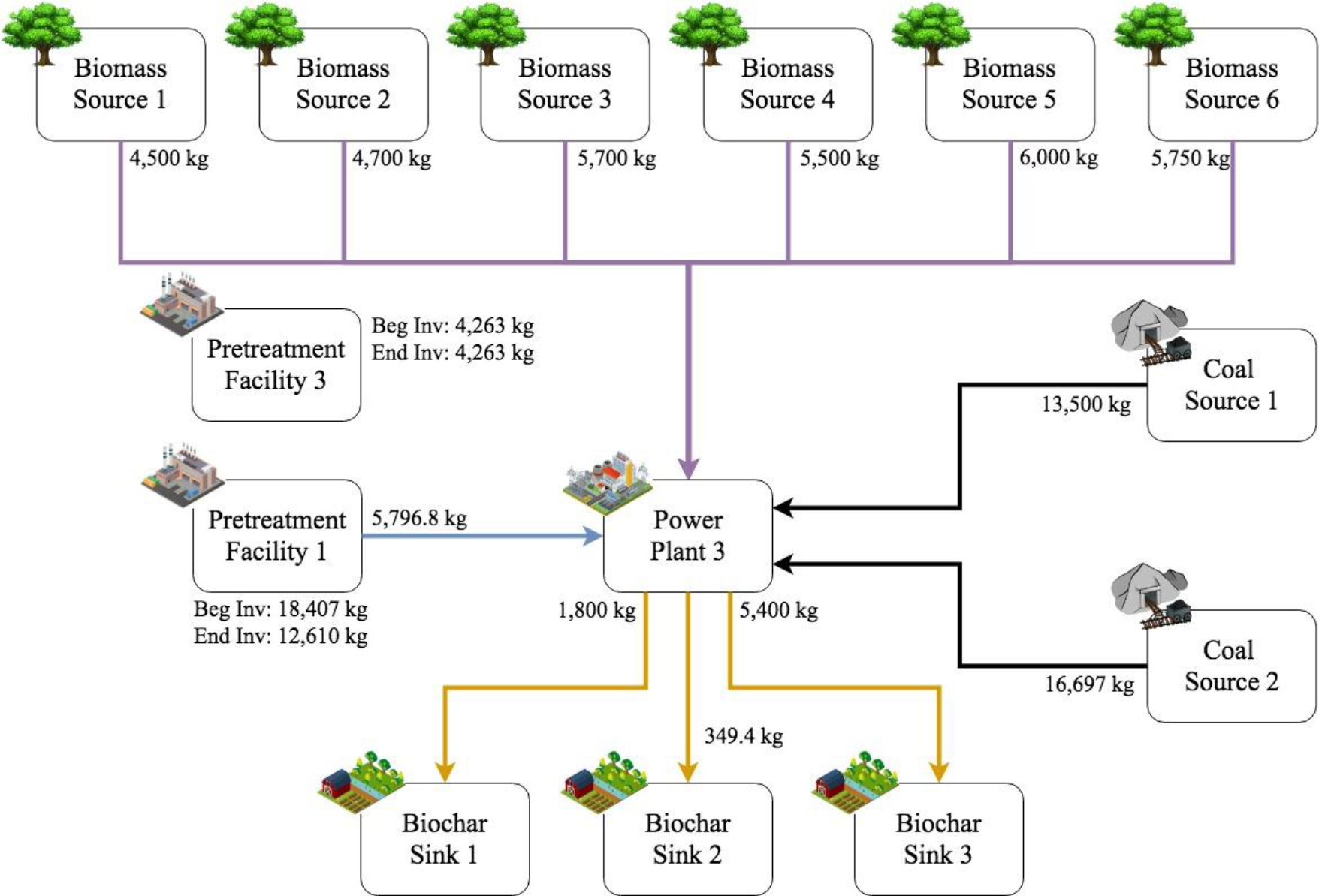
The optimal network for the first period is shown in Figure 2. The violet connection lines represent the flow of raw biomass from biomass sources to coal power plants, while the green connection lines represent the movement of raw biomass from biomass sources to pretreatment facilities. The movement of biomass after treatment and/or storage in pretreatment facilities to coal power plants are shown as blue arrows. Coal being brought from coal sources to coal power plants are illustrated as black lines. Lastly, the flow of biochar from power plants to biochar sinks are represented as yellow connection lines. The amount of material that flows between each node is indicated by the start of the connection arrows. It can be observed that raw biomass is purchased from all sources, some were directed towards pretreatment facilities. However, pretreated biomass is kept in inventory. Only two out of three potential pretreatment facilities were activated. This shows that the model prioritizes the facilities which can improve the biomass’ quality the most, while also causing the least pollutant emissions and at least cost. No material flows occur between pretreatment facilities and coal power plants to prepare for the higher power demand in succeeding periods. In Figure 2, biomass is accumulated in pretreatment facilities in period 1, the same behaviour was observed in period 2. However, by the third period, illustrated in Figure 3, the biomass that was previously stored in the pretreatment facilities start to be brought and utilized by the power plants. In addition, the model decides to divide satisfying the demand between three power plants, instead of having just one power plant to satisfy the whole demand for the first period, to avoid significantly decreasing the conversion efficiency of these coal power plants, which could later increase costs and emissions when more feedstock is needed to satisfy future demand, or when repairs would have to be made. Finally, all three power plants allocate biochar to sink 3 because it has the highest sequestration factor which offsets the carbon emissions from being farther from the power plants and having lower contaminant limits. In succeeding periods, the model is observed to choose expanding capacity, and performing maintenance on damaged equipment. Moreover, pretreated biomass is utilized to avoid damaging the equipment any further, and to be able to satisfy more demand from improved conversion efficiency.
The deterministic optimal solution is tested against uncertain levels of biomass moisture and ash content through Monte Carlo simulation. The optimal solution obtained in the deterministic base run is set as fixed parameters and is tested with 150 samples of randomly varying levels of biomass moisture and ash content to determine the robustness of the solution, and its ability to satisfy requirements under realizations of uncertainties. The results of the Monte Carlo simulation for the amount of demand satisfied and probability of meeting demand are summarized in Table 12. Varying the biomass properties while keeping the decision variables values as parameters created erratic results for the amount of electricity that could be generated each period. For all five periods, the system experiences difficulty in trying to meet the demand. Additionally, the performance of the model on its cost objective when subjected to uncertainty is also erratic. The objective costs can vary greatly from USD 1.532 to 1.605 million, with an average of USD 1,557,993.66, which is significantly higher than USD 1,535,762.55 obtained from the deterministic model.
Optimal network for period 1 of deterministic model
Optimal network for period 3 of deterministic model
Monte Carlo simulation results on demand satisfaction
| Period [year] | Demand [MJ] | Average demand satisfied [MJ] | Probability |
| 1 | 500,000 | 495,393.93 | 0.2933 |
| 2 | 600,000 | 593,669.20 | 0.2533 |
| 3 | 550,000 | 545,768.07 | 0.2800 |
| 4 | 600,000 | 600,793.93 | 0.5600 |
| 5 | 540,000 | 539,740.20 | 0.5133 |
| Average | 0.2533 |
Although the deterministic model performed well, it only did so because of known and certain biomass properties, particularly moisture and ash content. In real scenarios, decision makers are faced with the difficulty of making proper investment decisions and properly allocating biomass and coal feedstock and biochar to their appropriate sinks to satisfy demand at minimum cost and emissions while influenced by unknown and uncertain biomass moisture and ash content. Thus, to address an oversight of existing literature, this study proposes the use of TORO approach to reconcile and consider the tradeoffs of uncertain biomass properties with multi-objective biomass co-firing network design and optimization. This approach only requires the decision maker to provide an upper and lower limit of estimation for the uncertain parameters to which the model will return a robust solution. In addition, this approach balances the tradeoffs between a certain level of risk the decision maker is willing to tolerate or conservativeness without having to give up too much of the optimal solution for a robust solution.
In the model implementation, several values of were considered in increments of 0.1, providing 11 targets for both costs and environmental emissions using eq. (72) and eq. (73). Then, a solution is obtained for each of the targets through a bisection search maximizing the robustness index θ. The targets obtained from this is shown in Table 13.
Robust solution and Monte Carlo simulation results
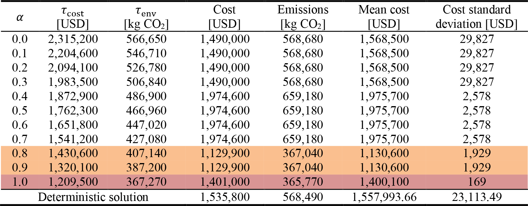 |
Each of the 11 solutions obtained were also subjected to biomass moisture and ash content uncertainty through the Monte Carlo simulation. Table 13 presents the specific costs and emissions targets for each σ value, and shows the maximum robustness index, which describes the amount of uncertainty the model is protected against, achieved for each of the 11 solutions. The operational objective values obtained from each of the 11 TORO solutions, as well as the mean and standard deviations of the cost from the Monte Carlo simulation are also shown. The mean and standard deviation of the cost objective was taken for each of the 150 data points generated for each σ level to provide a basis for comparison, which would allow non-dominated solutions to be identified. The standard deviation shows how much the solution may deviate from the mean in case of uncertainty. This value can represent how robust a solution is. A solution can be considered as superior if it is able to offer a lower average and standard deviation for costs. It can also be observed that there are some points which perform well on one metric but poorly on the other, while other points perform desirably on both. The solutions obtained when σ = 0.8 and 0.9 and when σ = 1.0 are the best solutions since they provide the lowest mean costs and standard deviation. The average costs when σ = 0.8 and 0.9 (USD 1,130,600) is significantly lower than the deterministic average (USD 1,557,993.66). On the other hand, mean costs when σ = 1.0 (USD 1,400,100) is slightly higher than the average costs for σ = 0.8 and 0.9, but can still found well below the deterministic solution and deterministic mean. The solution obtained when σ = 0.0 to 0.3, has lower mean costs than when σ = 0.4 to 0.7, but results in higher cost standard deviation. Regardless, these two solutions performed worse than the deterministic solution.
Solutions under σ-values 0.8 to 1.0 dominates all the others on all metrics. These solutions produce operational cost and emission values, mean costs, and cost standard deviation that are lower or better than the deterministic solution. However, when choosing between the two solutions, namely the solution for σ-values 0.8 to 0.9 (highlighted in green) and the solution for σ-value 1.0 (highlighted orange), a decision maker who prioritized costs over environmental emissions may find the former more attractive because of its lower mean costs, despite contributing higher operational pollutant emissions. On the other hand, if the environmental objective is more important to the stakeholders, the latter solution might be a better option. Furthermore, this solution might be more attractive because lower cost standard deviation was obtained from the Monte Carlo simulation, despite having higher mean costs than the solution when σ-value is 0.8 or 0.9. Thus, the decision maker would have to consider which among the metrics, operational emissions, mean costs, and standard deviation, carry the most weight for them.
The simulation reveals that the TORO approach is able to produce solutions for the model that are strictly better than the optimal solution obtained from the deterministic approach. In fact, the deterministic model returned costs and emissions that are much higher when subjected to biomass quality uncertainty compared to the robust solution. With the TORO approach, the decision maker does not need to know the actual distribution or level of biomass moisture and ash contents, and does not sacrifice too much of the optimality in the solution when maximizing robustness.
A novel multi-objective mixed integer non-linear programming model was developed for biomass co-firing supply networks with biochar carbon management networks that ensures robustness to biomass quality uncertainty, while ensuring that economic and environmental targets are satisfied. The model covers investment, production, and distribution planning, while accounting for the impact of feedstock properties throughout the supply chain. The proposed MOTORO model uses the robustness index θ to measure the design’s vulnerability to fluctuations in critical parameters. Model capabilities are demonstrated using an illustrative case study. The proposed robust model identifies solutions that are relatively more immune to realizations of biomass quality uncertainty depending on the risk-appetite of the decision maker. The model may be useful to stakeholders, such as network designers and managers, to commit to a final network design. Policies may then be drafted by prioritizing designs that satisfy robustness and objective targets. Future work may consider the extension of the multi-objective consideration to simultaneously account for other sustainably measures, such as other environmental impacts and social impact. Moreover, biomass is a flexible energy source, thus other bioenergy and bioproducts may be integrated into the model. Lastly, the model and its extensions may be applied to real-world and commercial-scale problems.
| Alt | binary, 1 if coal power plant l is operating on period t | [-] |
| ac | ash content of coal | [%] |
| ash content of raw biomass from source i on period t | [%] | |
| maximum allowable ash content in coal power plant l | [%] | |
| minimum allowable ash content in coal power plant l | [%] | |
| ash content of pretreated biomass in pretreatment facility k on period t | [%] | |
| ash content of all biomass in coal power plant l on period t | [%] | |
| ash content of feedstock in coal power plant l on period t | [%] | |
| accumulated excess ash content of feedstock in coal power plant l on period t | [%] | |
| accumulated ash content insufficiency of feedstock in coal power plant l on period t | [%] | |
| Bkt | binary, 1 if pretreatment facility k undergoes storage capacity expansion on period t | [-] |
| blnt | amount of biochar produced and transported from power plant l to biochar sink n on period t | [kg] |
| bpit | cost of biomass from source i on period t | [USD] |
| Clt | binary, 1 if coal power plant l undergoes capacity expansion on period t | [-] |
| ce | emissions due to coal combustion | [kg CO2/kg] |
| cpjt | cost of coal from source j on period t | [USD] |
| Dt | amount of energy demanded on period t | [MJ] |
| distance from biomass source i to pretreatment facility k | [km] | |
| distance from pretreatment facility k to coal power plant l | [km] | |
| distance from biomass source i to coal power plant l | [km] | |
| distance from coal source j to coal power plant l | [km] | |
| distance from coal power plant l to biochar sink n | [km] | |
| DP | penalty cost for unmet demand | [USD] |
| Elt | accumulated feedstock processed in coal power plant l on period t | [kg] |
| capacity expansion for processing biomass in pretreatment facility k on period t | [kg] | |
| capacity expansion for storage in pretreatment facility k on period t | [kg] | |
| capacity expansion for coal power plant l on period t | [kg] | |
| Fkt | binary, 1 if pretreatment facility k is operating on period t | [-] |
| fixed cost to expand the capacity of pretreatment facility k on period t | [USD] | |
| fixed cost to expand the storage capacity of pretreatment facility k on period t | [USD] | |
| fixed cost to expand the capacity of coal power plant l on period t | [USD] | |
| fhkt | fixed cost to store in pretreatment facility k on period t | [USD] |
| fml | fixed cost to repair/perform maintenance on the equipment in coal power plant l | [USD] |
| Gn | sequestration factor of biochar sink n | [-] |
| gf | biochar yield from co-firing scheme f | [-] |
| hcl | concentration of contaminant c in the biochar produced in power plant l | [g/kg] |
| maximum allowable concentration of contaminant c in biochar sink n | [g/kg] | |
| Ikt | ending biomass inventory in pretreatment facility k on period t | [kg] |
| J | biochar application cost | [USD] |
| Kf | severity of damage in equipment due to co-firing scheme f | [USD] |
| lower coal displacement limit of coal power plant l retrofitted for co-firing scheme f | [km] | |
| upper coal displacement limit of coal power plant l retrofitted for co-firing scheme f | [km] | |
| moisture content of raw biomass from source i on period t | [%] | |
| mc | moisture content of coal | [%] |
| maximum allowable moisture content in coal power plant l | [%] | |
| minimum allowable moisture content in coal power plant l | [%] | |
| moisture content of all biomass in pretreatment facility k on period t | [%] | |
| moisture content of all biomass in coal power plant l on period t | [%] | |
| moisture content of feedstock in coal power plant l on period t | [%] | |
| accumulated excess moisture content of feedstock in coal power plant l on period t | [%] | |
| accumulated moisture content insufficiency of feedstock in power plant l on period t | [%] | |
| Olft | binary, 1 if coal power plant l retrofitted for co-firing scheme f is used on period t | [-] |
| odt | energy produced over demand on period t | [MJ] |
| Pkt | binary, 1 if pretreatment facility k undergoes processing capacity expansion on period t | [-] |
| bulk density of raw biomass from source i on period t | [kg/m3] | |
| pc | bulk density of coal | [kg/m3] |
| bulk density of pretreated biomass in pretreatment facility k on period t | [kg/m3] | |
| pb | bulk density of biochar | [kg/m3] |
| pckt | biomass pretreatment cost in facility k on period t | [USD] |
| pekt | emissions due to biomass pretreatment in facility k on period t | [kg CO2/kg] |
| qc | lower heating value of coal | [kJ/kg] |
| lower heating value of biomass in coal power plant l on period t | [kJ/kg] | |
| qlt | lower heating value of feedstock in coal power plant l on period t | [kJ/kg] |
| qlf | binary, 1 if coal power plant l is retrofitted for co-firing scheme f | [-] |
| rlt | repair/maintenance effectiveness in coal power plant l on period t | [-] |
| Skt | binary, 1 if storage in pretreatment facility k is used on period t | [-] |
| amount of biomass available at biomass source location i on period t | [kg] | |
| amount of coal available a coal source location j on period t | [kg] | |
| Tn | total biochar storage capacity of sink n | [kg] |
| number of trips to transport raw biomass from source i to pretreatment facility k on period t | [-] | |
| number of trips to transport treated biomass from facility k to power plant l on period t | [-] | |
| number of trips to transport raw biomass from source i to power plant l on period t | [-] | |
| number of trips to transport coal from source j to coal power plant l on period t | [-] | |
| number of trips to transport biochar from coal power plant l to sink n on period t | [-] | |
| tc | transportation costs per unit distance per trip | [USD] |
| te | transportation emissions | [kg CO2/kg] |
| U | transport weight capacity | [kg] |
| Unit capacity expansion cost of pretreatment facility k on period t | [USD] | |
| unit storage capacity expansion cost of pretreatment facility k on period t | [USD] | |
| unit capacity expansion cost of coal power plant l on period t | [USD] | |
| uhkt | unit holding cost in pretreatment facility k on period t | [USD] |
| uml | unit cost of repair/maintenance on the equipment in coal power plant l per unit efficiency | [USD] |
| uk | ash content improvement efficiency in pretreatment facility k | [-] |
| udt | unmet demand on period t | [MJ] |
| V | transport volume capacity | [kg3] |
| vk | moisture content improvement efficiency in pretreatment facility k | [-] |
| Wlt | binary, 1 if coal power plant l is repaired/undergoes maintenance on period t | [-] |
| wikt | amount of biomass transported from biomass source i to pretreatment facilities k on period t | [kg] |
| Xkt | new weight of biomass from source after pretreatment in facility k on period t | [kg] |
| xklt | amount of biomass transported from pretreatment facilities k to power plant l on period t | [kg] |
| combustion capacity of coal power plant l on period t | [kg] | |
| pretreatment capacity in facility k on period t | [kg] | |
| storage capacity in pretreatment facility k on period t | [kg] | |
| yilt | amount of biomass transported from biomass source i to coal power plant l on period t | [kg] |
| zjlt | amount of coal transported from coal source j to coal power plant l on period t | [kg] |
| Greek letters | ||
| βl | efficiency threshold of coal power plant l | [-] |
| γ | conversion factor for heat energy to electrical energy | [-] |
| ψ | allowable soil contaminant tolerance factor | [-] |
| γlt | efficiency loss of equipment in coal power plant l on period t | [-] |
| Subscripts and superscripts | ||
| c | biochar contaminant types | |
| f | co-firing scheme | |
| i | biomass waste source | |
| j | coal source | |
| k | biomass pretreatment facility | |
| l | coal power plant | |
| n | biochar sink | |
| t | time period | |
- ,
Integrating Biomass Into Energy Supply Chain Networks ,Journal of Cleaner Production , Vol. 248 ,pp 119246 , 2020, https://doi.org/https://doi.org/10.1016/j.jclepro.2019.119246 - ,
Multi-Site and Multi-Period Optimization Model for Strategic Planning of a Renewable Hydrogen Energy Network from Biomass Waste and Energy Crops ,Energy , Vol. 185 ,pp 527-540 , 2019, https://doi.org/https://doi.org/10.1016/j.energy.2019.07.053
AvisoK. B.
San JuanJ. G.
SyC. L.
TanR. R.
Optimal Planning of Biomass Co-Firing Networks with Biochar-Based Carbon Sequestration
Advances in Carbon Management Technologies
342-355
CRC Press
Boca Raton, Florida, USA
2020
- ,
Life Cycle Environmental Impact Assessment of Fuel Mix-Based Biomass Co-Firing Plants with CO2 Capture and Storage ,Applied Energy , Vol. 252 ,pp 113483 , 2019, https://doi.org/https://doi.org/10.1016/j.apenergy.2019.113483 - ,
Data-driven Wasserstein Distributionally Robust Optimization for Biomass with Agricultural Waste-to-Energy Network Design Under Uncertainty ,Applied Energy , Vol. 255 ,pp 113857 , 2019, https://doi.org/https://doi.org/10.1016/j.apenergy.2019.113857 - ,
Development and Application of a Decision Support Tool for Biomass Co-Firing in Existing Coal-Fired Power Plants ,Journal of Cleaner Production , Vol. 236 ,pp 117375 , 2019, https://doi.org/https://doi.org/10.1016/j.jclepro.2019.06.206 - ,
A Review of Biomass Co-Firing in North America, Renewable and Sustainable Energy Reviews , Vol. 40 ,pp 930-943 , 2014, https://doi.org/https://doi.org/10.1016/j.rser.2014.07.195 - ,
Biomass as an Energy Source in Coal Co-Firing and its Feasibility Enhancement via Pre-Treatment Techniques ,Fuel Processing Technology , Vol. 159 ,pp 287-305 , 2017, https://doi.org/https://doi.org/10.1016/j.fuproc.2017.01.029 - ,
A Multi-period Source-sink Mixed Integer Linear Programming Model for Biochar-Based Carbon Sequestration Systems ,Sustainable Production and Consumption , Vol. 8 ,pp 57-63 , 2016, https://doi.org/https://doi.org/10.1016/j.spc.2016.08.001 - ,
Biochar Systems in the Water-Energy-Food Nexus: The Emerging Role of Process Systems Engineering ,Current Opinion in Chemical Engineering , Vol. 18 ,pp 32-37 , 2017, https://doi.org/https://doi.org/10.1016/j.coche.2017.08.005 - ,
Models for Optimization and Performance Evaluation of Biomass Supply Chains: An Operations Research Perspective ,Renewable Energy , Vol. 87 (2),pp 977-989 , 2016, https://doi.org/https://doi.org/10.1016/j.renene.2015.07.045 - ,
Spatial Optimisation of Oil Palm Biomass Co-Firing for Emissions Reduction in Coal-Fired Power Plant ,Journal of Cleaner Production , Vol. 172 ,pp 3428-3447 , 2018, https://doi.org/https://doi.org/10.1016/j.jclepro.2017.11.027 - ,
Availability of Biomass Residues for Co-Firing in Peninsular Malaysia: Implications for Cost and GHG Emissions in the Electricity Sector ,Energies , Vol. 7 (2),pp 804-823 , 2014, https://doi.org/https://doi.org/10.3390/en7020804 - ,
Optimization of Pre-Treatment Selection for the Use of oody Waste in Co-Combustion Plants ,Chemical Engineering Research and Design , Vol. 92 (8),pp 1539-1562 , 2014, https://doi.org/https://doi.org/10.1016/j.cherd.2014.01.004 - ,
A Multi-Objective Optimization Model for the Design of Biomass Co-Firing Networks Integrating Feedstock Quality Considerations ,Energies , Vol. 12 (12),pp 2252 , 2019, https://doi.org/https://doi.org/10.3390/en12122252 - ,
A Multi-Objective Optimization Model for the Design of a Biomass Co-Firing Supply Network ,Chemical Engineering Transactions , Vol. 70 ,pp 223-228 , 2018, https://doi.org/https://doi.org/10.3303/CET1870038 - ,
and Optimization of Biomass Supply Chains: A Review and a Critical Look ,IFAC-PapersOnLine , Vol. 49 (12),pp 604-615 , 2016, https://doi.org/https://doi.org/10.1016/j.ifacol.2016.07.742 - ,
Effects of Biochar Application on Soil Greenhouse Gas Fluxes: A Meta-Analysis ,GCB Bioenergy , Vol. 9 ,pp 743-755 , 2017, https://doi.org/https://doi.org/10.1111/gcbb.12376 - ,
Bi-Objective Optimization of Biochar-Based Carbon Management Networks ,Journal of Cleaner Production , Vol. 188 ,pp 911-920 , 2018, https://doi.org/https://doi.org/10.1016/j.jclepro.2018.04.023 - ,
Biomass Supply Chain Network Design: An Optimization-riented Review and Analysis ,Industrial Crops and Products , Vol. 94 ,pp 972-1000 , 2016, https://doi.org/https://doi.org/10.1016/j.indcrop.2016.09.027 - ,
Integrating Biomass Quality Variability in Stochastic Supply Chain Modeling and Optimization for Large-Scale Biofuel Production ,Journal of Cleaner Production , Vol. 149 ,pp 904-918 , 2017, https://doi.org/https://doi.org/10.1016/j.jclepro.2017.02.123
JuanSan
SyJ. L.
L.C.
Multi-Objective Robust Optimization for the Design of Biomass Co-firing Networks
Proceedings of the Asia Pacific Industrial Engineering & Management Systems Conference 2018
Hong Kong
December 5-8
2019
- ,
An Affine Adjustable Robust Model for Generation and Transmission Network Planning ,Electrical Power and Energy Systems , Vol. 60 ,pp 141-152 , 2014, https://doi.org/https://doi.org/10.1016/j.ijepes.2014.02.026 - ,
Biomass Quality Control in Power Plants: Technical and Economical Implications ,Renewable Energy , Vol. 115 ,pp 908-916 , 2018, https://doi.org/https://doi.org/10.1016/j.renene.2017.09.026 - ,
Property Analysis and Pretreatment of Rice Straw for Energy Use in Grain Drying: A Review ,Agriculture and Biology Journal of North America , Vol. 1 (3),pp 195-200 , 2010, https://doi.org/https://doi.org/10.5251/abjna.2010.1.3.195.200 - ,
Energy from Combustion of Rice Straw: Status and Challenges to China ,Energy and Power Engineering , Vol. 3 (3),pp 325-331 , 2011, https://doi.org/https://doi.org/10.4236/epe.2011.33040
BainsM.
RobinsonL.
Material Comparators for End-of-Waste Decisions ‒ Materials for Fuels: Coal
Environment Agency
Bristol, UK
2016