Nowadays the environmental impact of free trade and energy use has been the main focus of researchers and policymakers. This is because it has been found that trade and energy use have a significant impact on measures of environmental pollution like carbon dioxide (CO₂) [1], sulfur dioxide (SO₂) [2], particulate matter (PM10) [3], and the overall greenhouse gas (GHG) emissions [4].

In the literature of trade and the environment three main channels by which trade can assert its impact on the environment are; the scale, technique, and composition effects. These channels have been thoroughly elaborated by [5] and [6]. According to [7], the entire effect of trade on the environmental pollutants depends on a combination of increasing income, technological innovation, and changes in the composition of the industry. Empirical studies by [8] and [9] among others have reaffirmed that gross domestic product (GDP) is the main driver of CO₂ emissions. The scale effect, therefore, demonstrate that increase in income is associated with increased emissions. While the technique effect refers to the beneficial effect of high income caused by trade openness, change in the technique of production, and people’s demand for environmental quality and protection. It is believed that at a higher income level, trade openness may result in high technology imports leading to lower emissions per unit of output. With the composition effect, trade can increase emissions and degraded the environment. This is because with an increased income and structural transformation from agriculture to industrial sector emissions may likely increase. It has been argued that the composition effect depends on whether a country has a competitive advantage in dirtier or cleaner production [10]. With this argument, it is uncertain that, the composition effect can increase or decrease environmental pollution [11]. This is because the effect can lead to decrease emissions if growing industries are technology-driven. Also if the structural transformation necessitated by trade and growth, is from the industry to services sector emissions would be expected to decrease [12].

It is important to note that the consumption of energy is a key determinant of CO₂ emissions and environmental degradation. The environmental damages caused by the consumption of energy are mostly driven by the use and exploitation of fossil fuel energy resources [13]. There is sufficient empirical evidence pointing that energy consumption is the main cause of CO₂ emissions [14], particulate matter (PM10) [15], sulfur dioxide (SO₂) [16], and overall GHG emissions [4]. From 2000–2010 GHG emissions grew rapidly which was a result of high energy demand from fossil fuel sources [17]. According to [18] the growth in CO₂ emissions was stagnated from the year 2014–2016 because of low carbon emissions technology and improved energy efficiency. Meanwhile, in 2017 global CO₂ emissions related to energy consumption increased by 1.7% [18], and the African continent is no exception to this increase. This is because the continent is rich with energy resources accompanied by increasing demand for energy-related resources. Africa relied more on conventional fossil fuel energy which has a more damaging effect on the environment and represents about 40% of the total energy mix in the continent [19]. In terms of growth in the energy demand, the continent is becoming an important driver of world energy usage growth because of its abundant fossil fuel, minerals, and solar power-related energy resources [19]. Despite Africa’s low contribution to the global carbon emissions related to energy use which is estimated at 2%, the continent is extremely closer and more susceptible to global climate change [19]. The continent’s energy intensity exceeds the global average and specifically above that of the Organization of Economic Cooperation and Development (OECD) countries [18]. It has been reported that over 90% of African countries used non-renewable energy [20]. This has made the continent of special interest in analyzing energy effects on CO₂ emissions and environmental degradations.

The effect of trade and energy use on emissions and environmental degradation can be analysed using the environmental Kuznets curve (EKC) model. This is because the model is based on the relationship between GDP and environmental pollution and works based on the scale, technique, and composition effects. According to this model at the initial stage of countries’ development, the scale and the composition effect exceed the technique effect. As the economy grows further a threshold point may be reached in which technique effect will dominate and this leads to decrease emissions and improve environmental quality. It is believed that trade is the driving force in shaping the pattern of EKC [21] by enabling the use of an energy-efficient technique of production which lowers environmental pollution. On the empirical ground, there is no valid evidence on the positive or negative consequence of free trade on environmental pollution [15]. It has been argued that for developing countries like Africa the scale and composition effects may dominate the technique effect. This is because for African countries the focus has been more on income growth, investment, and employment with little focus on environmental quality and protection. This may result in the phenomenon called the pollution haven hypothesis (PHH) in most developing countries. According to this hypothesis, trade may result in a pollution haven in poor and developing countries with weak environmental regulations. This is because, with trade openness, polluting industries in their bid to avoid the higher environmental cost in developed countries will tend to migrate to poor and developing countries with weak environmental regulations [22]. In this vein, therefore, as polluting industries move to poor and developing countries, poor and developing will become pollution haven with more pollution-intensive industries producing for export to developed countries [23]. Based on this hypothesis environmental quality would be improved in developed countries when open to trade and detriment in poor and developing countries. On the contrary, the factor abundance hypothesis posits that trade allowed countries to shift resources in areas that they possessed a comparative advantage [6]. Based on this hypothesis developed countries that are rich in capital stock will specialize in pollution-intensive export and production and become dirtier whereas developing countries with labour abundance will be specialized in labour-intensive export and production that are less polluting.

While incorporating various determinants of environmental pollutants within the EKC model, many scholars have explored the effect of trade and energy on different measures of environmental pollution in the context of different countries, different periods, and different methodologies. For instance, while examining the nexus between trade and CO₂ emissions in a panel of low, middle, and high-income countries [24], report that trade increases carbon emissions. While in the case of China [15] has found trade to decrease haze pollution (PM_2.5). A contradictory finding by [25] has shown that trade increases haze pollution in China over the period 2013–2017. A study by [26] has found trade to increase carbon emissions and reduces emissions by mediating growth and the level of industrialization in a panel of 181 countries. In 46 Sub-Saharan Africa [20] and 8 South Asian countries [27] revealed that trade and GDP increase CO₂ emissions while renewable energy reduces emissions. In the context of Nigeria and South Africa [28] has found an asymmetric effect of trade, renewable energy, and GDP on CO₂ emissions over the period 1990-2014. Studies by [29] and [30] report that trade and renewable energy reduces CO₂ emissions in India, Brazil, and South Africa while GDP growth increases emissions in India and reduces them in Brazil and South Africa. Similarly, [31] observed that trade and renewable energy consumption reduces ecological footprint while GDP degrades the environment by increasing the ecological footprint in South Africa. Another study [4] also concludes that trade openness, renewable energy, and energy efficiency reduce GHG emissions while GDP and industrialization increase GHG emissions and detriment the environment.

A study by [1] reports that trade openness, GDP growth, and energy consumption rises CO₂ emissions and degrade the environment in Sub-Saharan Africa. A similar finding has been reported by [32] in the Middle East and North Africa (MENA) countries, [11] in Tunisia, and [33] in the Asia Pacific Economic Cooperation. Contrarily, [34] revealed that trade openness reduces CO₂ emissions while GDP and energy use increases CO₂ emissions in the Organization of Petroleum Exporting Countries (OPEC). A study by [7] also has found trade openness, GDP, and capital-labour ratio to significantly influence localized environmental pollutants. In the case of Malaysia, [35] reports that the trade and capital-labour ratio reduces CO₂ emissions while GDP and energy consumption increases CO₂ emissions. Contrary to this finding [36] observed that trade and capital stock increase emissions in European Union and the Persian Gulf regions. A similar finding has also been reported by [37] in Tunisia and Morocco. [38], analysed the dynamic effect of trade openness, GDP, energy use, and capital-labour ratio on CO₂ emissions in South Africa. Their finding indicates that these variables increase CO₂ emissions and detriment the environment. [39], investigate the effect of globalization, GDP growth, energy use, and democracy on carbon emissions in South Africa and report that globalization and energy consumption increases emissions while democracy reduces carbon emissions. [40], revealed that energy use increases CO₂ emissions while democratic government reduces emissions in India. While analysing the macroeconomic determinants of CO₂ emissions in Nigeria [41], report no evidence of trade effect on CO₂ emissions while GDP increases CO₂ emissions and that energy use and manufacturing value-added reduces CO₂ emissions. Contrarily [42] observed that imports, GDP growth, coal consumption, and industrialization increase CO₂ emissions while exports decrease emissions and improve the environment in Turkey. The case of Indonesia also [43] indicates that trade, GDP growth, and industrialization degrade the environment by increasing coal consumption.

Empirical studies based on input-output (I-O) models and econometric techniques have demonstrated different channels by which countries can become a pollution haven. For instance, a study by [44] supports PHH in MENA countries. [45], also revealed that China is a pollution haven resulting from its trade with North America, Western Europe, and other developed regions whereas its CO₂ emissions outflow were embodied in its trade with Sub-Saharan Africa, South Asia, and America. A study by [46] reports that South African Customs Union countries’ are having pollution from trade with the United States and the United Kingdom. In the context of the computable general equilibrium model [47] has observed that developed countries tend to shift their polluting activities to poor and developing countries while a contradictory finding by [48], revealed that SO₂ emissions embodied in trade flew from developing to developed countries. another study by [49] has found little evidence that trade leads to environmental burden shift from developed to developing countries. [50], has found that trade significantly transfers pollution across 151 OECD and non-OECD economies. [51], reports that trade significantly affects emissions embodied in Chinese export to developed countries. Over the period 1990-2015 [52] show that Hong Kong is the net importer of CO₂ emissions. Using the pollution term of trade (PTT) indicator [53] have found that China’s PTT is greater than 1 implying that China produces more emissions to obtain a given unit of value-added exports than its trading partners. Studies by [54] and [55] analysed the case of China-Russia and China-India trade and show that China is the net exporter of pollution-intensive goods to Russia and India and became a pollution haven in trading with these countries.

Therefore, within the EKC hypothesis, the present study aims to examine the effect of goods trade and energy on environmental pollution in African countries. This is important because African countries have been characterized by alarming environmental issues and there is a need to understand the forces behind these environmental problems. The continent is more susceptible to environmental degradation owing to the energy-related problem, rapid population growth, illiteracy, and political uprising. Despite these problems, Africa remained the least in terms of contribution to global CO₂ emissions which is less than 5% of the global emissions [56]. This has resulted in little attention given to the environmental consequences of free trade and energy on the continent. Therefore, Africa is an important case of understanding the role of trade and energy in generating carbon emissions and environmental degradation. This is because since the 1970s emissions have been consistently increasing and the continent is no exception in that regard. So also, empirical studies on the environmental consequences of free trade were mainly focused on the overall trade with little focus on the goods trade that is considered more polluting. A study by [57] report that goods production has been the greatest cause of CO₂ emissions and that more than 50% of world outputs are exchanged internationally [58]. Therefore, there is a need to provide an understanding of the specific effect of goods trade on the environment in African countries. This is because African countries are more open to merchandise trade than services. The continent has been a market for other regions’ manufactured goods and a key player in primary product exports which are extracted from available endowed resources and likely to degrade the environment.

This study, therefore, contributes in many ways to the debate on the environmental impact of trade and energy use. We proposed an empirical model that was formulated based on the different channels through which trade affects environmental pollution. We decompose the effect of trade into the scale, technique, and composition effects using the EKC model. We further examined and incorporated a cubic component into the model of EKC to determine whether the turning of EKC (if exist) is only temporary. We also recognized the role of the turning point in the trade and CO₂ emissions nexus. We empirically investigate the degree to which African countries become pollution haven based on income and factor comparative advantage. Available studies on African countries do not investigate this impact. Of interest to this study are GDP, trade, energy, and capital-labour ratio which we considered as the determinants of environmental degradation. One vital methodological issue addressed in this study is the way trade openness is measured. We constructed an openness index based on the [59] approach. This is a complete departure from previous work that applied the traditional trade/GDP ratio despite its weakness and assessed the environmental impact of free trade. Therefore, our study provides a more precise estimate of the effect of trade on the environmental quality measure as CO₂ emissions.

Following empirical studies in energy and environmental economics, this study examines the role of goods trade and energy in generating CO₂ emissions and environmental degradation. We developed an empirical model within the EKC hypothesis. The carbon emissions function used in this study and the explanatory and control variables incorporated into the model were in line with most of the existing literature in trade, energy, and environmental economics. The panel specification of trade and energy impact on emissions is expressed in Equation (1) as follows:

$lnC{O}_{2it}={\text{δ}}_0+{\text{δ}}_{1}ln{Y}_{it}+{\text{δ}}_{2}ln{Y}_{it}{}^2+{\text{δ}}_{3}ln{Y}_{it}{}^3+{\text{δ}}_{4}lnT{O}_{it}+{\text{δ}}_{5}lnT{O}_{it}{}^2+{\text{δ}}_{6}lnK{L}_{it}+{\text{δ}}_{7}lnE{N}_{it}+{\varphi }_1{X}_{ir}+v_i+{\eta }_t+{\epsilon }_{it}$ (1)

where subscripts denote: i – country dimension, t – the period, CO₂ is carbon emissions a proxy of environmental degradation, Y is the per capita real GDP which measures the scale effect, Y² is the square of GDP which measures the technique effect, Y³ is the cubic component incorporated to verify whether the technique effect (if exists) is only temporary, TO is trade openness, TO² is the square of trade openness introduced to verify the non-linear nexus between trade and carbon emissions, KL is the capital-labour ratio which measures the composition effect, EN is the energy intensity which measures the energy effect, X is the vector of control variables which include democratic government, agriculture, industry, and services value-added, v_i isv_i the country-specific effect, η_t is the time effect, ε_it is the classical error term.

To investigate the indirect channels by which trade and energy affect the environment and to verify the pollution haven hypothesis (PHH) and factor abundance effect, we extend Equation (1) to include interaction terms of trade and GDP, trade and capital-labour ratio, and finally trade and energy intensity. Hence, our empirical model with interaction effects is expressed in Equation (2) as follows:

$lnC{O}_{2it}={\text{δ}}_0+{\text{δ}}_{1}ln{Y}_{it}+{\text{δ}}_{2}ln{Y}_{it}{}^2+{\text{δ}}_{3}ln{Y}_{it}{}^3+{\text{δ}}_{4}lnT{O}_{it}+{\text{δ}}_{5}lnT{O}_{it}{}^2+{\text{δ}}_{6}lnK{L}_{it}+{\text{δ}}_{7}lnE{N}_{it}+{\lambda }_1\ln T{O}_{it}\times \ln Y_{it}+{\lambda }_{2}T{O}_{it}\times \ln K{L}_{it}+{\lambda }_3\ln T{O}_{it}\times \ln E{N}_{it}+{\varphi }_1{X}_{ir}+v_i+{\eta }_t+{\epsilon }_{it},$ (2)

Where TO × Y is the variable which measures the income pollution haven effect i.e. PHH, TO × KL is the variable which measures the factor abundance effect, TO × EN, is the variable which measures the interaction effect of trade through energy intensity. δ₀ …δ₇, η₁…η₃ and ϕ₁ are the parameters to be estimated. All other variables are as defined in Equation (1).

Equations (1) and (2) can simply be estimated using pooled ordinary least square (POLS) provided that the error term ϕ is identically distributed and not correlated with the regressors i.e. Cor(ϕ_i,x_i) = 0. That is if we assume that there is no country effect (v_i), then Equations (1) and (2) become purely ordinary least square (OLS). Because of panel individual effect (v_i) in Equations (1) and (2) POLS may result in heterogeneity bias. To correct for this bias and to account for the time effects Equations (1) and (2) include three error component i.e. (v_i+η_t + ϕ_it) which accounts for both the country and time effect. With the three error component (v_i+η_t +ϕ_it), therefore, Equations (1) and (2) can be estimated using fixed effect (FE) and random effect (RE) models. RE model treat v_i as random and not correlated with the regressors. While the FE model assumed v_i to be constant but different across panel such that v_i = η_t and that η_t = 0 which yields a one-way FE model. In this study, therefore, we applied different assumptions regarding the behaviour of v_i + η_t and chose the most efficient estimate based on the Hausman specification test.

For the robustness checks, to our empirical findings, Equations (1) and (2) are also estimated using the dynamic generalized method of moment (GMM) approach. This is important because estimating the dynamic version of Equations (1) and (2) using FE and RE models may lead to bias estimates because it is likely that some explanatory variables are endogenous which can be controlled using the GMM approach.

In choosing the most efficient model two different tests are conducted. The Breusch-Pagan Lagrangian Multiplier (BP-LM) test for chosen between POLS and RE models and the Hausman test for choosing between FE and RE models. The result from the BP-LM test is significant at a less than 1% level for all the estimated models (i.e. p-value 0.0000 < 0.05). In this case, the null hypothesis that the random effect variance is zero is rejected i.e. RE model is preferred to the POLS model since there is a country effect in our panel. to treat the country effect we conducted the Hausman test. The chi-square statistics of the test is statistically insignificant for all the estimated models (1)–(6) i.e. p-values of the chi-square obtained are all greater than 0.05. In this case, the null hypothesis of no correlation between the country's effects and regressors is accepted against the alternative hypothesis. Therefore, the FE model cannot be estimated, and that the RE model is preferred. To make sure that our model did not suffer from the problem of multicollinearity, serial correlation, heteroskedasticity, cross-section dependence, and potential outliers we again conducted different diagnostic checks. In all the estimates of Table 1, the variance inflation factor (VIF) test shows that our models did not have a multicollinearity problem because the VIF values are all less than 6 (required standard value) and 10 (threshold value). We used panel corrected standard error with AR1 to simultaneously diagnose for both heteroskedasticity and serial correlation of the disturbance term. The p-values from the Pesaran test failed to reject the null hypothesis of cross-sectional independence in all estimates. Hence, our data is more appropriate for panel analysis. Our estimates are also free from the problem of potential outliers because we checked and removed outliers using Cook's distance outlier test.

Table 1 and Figure 1 present the static estimate of RE models validated by the Hausman specification test. Different linear and polynomial models are reported for more robustness checks of the empirical findings. Models (1) and (2) were the baseline models estimate of Equations (1) and (2). The estimated parameters have the correct sign as expected in most estimates.

The baseline model (1) of Table 1, the finding suggests that a 1% increase in GDP is associated with a 1.073% increase in CO₂ emissions and environmental degradation. After adding and removing the interaction effects of trade and control variables in models (2)–(6), almost the same magnitude of parameter estimate is obtained. From models (1)–(6) of Table 1, the result revealed that CO₂ emissions exhibit a positive scale effect and this is consistent with our expected theoretical a priori.

The coefficient GDP square which measures the technique effect is negative and statistically significant in all estimates. This finding suggests that further increase in income will be accompanied by a decrease in emissions in the panel of African countries. From models (1)–(3) of Table 1, findings revealed that a 1% increase in income resulting from the technique effect (GDP2) will reduce emissions and improve environmental quality by 0.0911%, 0.123%, and 0.0822% respectively.

The positive scale effect (GDP) and negative technique (GDP²) effect as obtained in Table 1 validates the inverted U-shaped EKC hypothesis in all estimates. The presence of the N-shaped curve is rejected. This is because, in Table 1, there is no evidence of a positive and significant effect of GDP cubic (GDP³) on emissions.

Figure 1

Parameters of static models (Random effect)

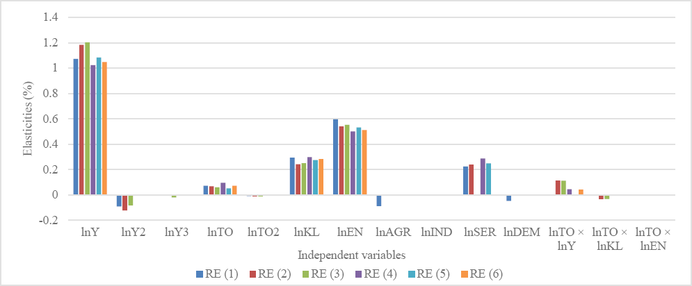
Our empirical finding is supported by many recent studies; [20] who observed positive scale and negative technique effects in a panel of 46 Sub-Saharan Africa, [27] in a panel of 8 South-Asian countries, and [32] in a panel of MENA countries among others. This finding implies that higher per capita income is associated with improved production techniques which lower carbon emissions and improve environmental quality. Albeit, the finding also indicates that the magnitude of the positive scale effect in all estimates of Table 1 is higher than the effect of the negative technique implying that the emission mitigation by the technique effect is not sufficiently large to offset the detrimental scale effect.

For the average African country, finding from Table 1 suggests that at less than 1% level the coefficient of trade openness is positive and statistically significant in all the estimated models. Other things being equal, higher openness in goods trade is associated with increased CO₂ emissions and environmental degradation. For instance, the baseline models (1) and (2) of Table 1 show that a 1% increase in trade openness is associated with a 0.0726% and 0.0683% increase in carbon emissions. This finding is consistent with the linear models (4)–(6) of Table 1 and supported by [1] and [20] finding both in a panel of 46 Sub-Saharan Africa and [26] in a panel of 181 countries among others. The finding also contradicts [29] finding in the context of Brazil, India, and South Africa, and [30] finding in the case of India. The detrimental effect of trade openness as observed in this study is attributed to Africa's primary products export that consume and relied more on resource extraction. This is because any rise in foreign demand resulting from market opening would result in high pressure on the use of environmental goods which increases emissions.

Also, the non-linear component of trade openness (TO²) indicates that there is a threshold point in which an increase in trade openness would result in decreased CO₂ emissions and improve environmental quality. This supports a non-linear inverted U-shaped nexus among trade and CO₂ emissions and consistent with [24] finding who in a sample of high-income countries observed an inverted U-shaped nexus between trade and CO₂ emissions. This observed inverted U-shaped in trade and emissions nexus is consistent with the verified EKC. This gave support that, the pattern of the EKC in African countries is determined by goods trade openness. A plausible explanation is that at the low level of openness, trade degrades the environment by increasing CO₂ emissions while at a high level, the trade will bring capital and technology for greener development in the continent.

In all the estimated models, looking at the elasticity of positive scale, composition, and trade openness effects. The beneficial technique effect in Table 1 is sufficiently weak to offset the detrimental scale, composition, and trade effects, and hence the net effect of trade openness is positive and detrimental to the environment.

In all the estimates, the finding revealed that the capital-labour ratio (KL) asserts a statistically significant increasing impact on CO₂ emissions at a less than 1% significance level. The positive composition effect indicates that with trade, capital is employed in more polluting sectors in African countries which increases CO₂ emissions and degrades the environment. From the baseline model (1) findings indicate that a 1% increase in capital relative to labour is accompanied by a 0.294% increase in CO₂ emissions and environmental degradation. Almost the same stable parameter estimate is obtained in all the polynomial and linear models of Table 1. This finding is supported by [7] finding who found the composition effect to increase emissions in a panel of 128 developed and developing countries and [38] in South Africa. The finding also contradicts [35] who found the composition effect to decrease CO₂ emissions in Malaysia and [36] in European Union and North-South region.

Furthermore, the result indicates a positive and significant effect of energy intensity on carbon emissions in all the estimates at less than a 1% level of significance. Finding from the baseline model (1) of Table 1 suggests that a 1% increase in energy use is associated with a 0.595% increase in CO₂ emissions and environmental degradation. Almost the same magnitude of a parameter is observed in all estimates of Table 1 with energy effect ranging between 0.500–0.595 percent increase in CO₂ emission. Based on the magnitude of the EN coefficient energy intensity is a key driver of CO₂ emissions and environmental degradation in African countries. The reason for the high energy effect is that the continent relied heavily on fossil fuels which is the major source of energy and the slow adoption rate of energy-efficient technologies and transfer to renewable energy sources. Another reason could be that the energy sector has been the major contributor TO GHG emissions in the continent. This finding is supported by [1] in the case of Sub-Saharan Africa, [27] in 8 South-Asian countries, [32] in MENA countries, and contradicts [41] in the case of Nigeria, and [44] in MENA countries among others.

We also confirmed the pollution haven hypothesis (PHH) in goods trade in all the estimated models. This is because the effect of trade through the level of development as captured by TO × Y is positive and statistically significant in all the estimates of Table 1. This finding suggests that African countries explore comparative advantage in pollution-intensive export and production. This is because developed countries with stringent environmental policies used trade openness as a means of transferring their polluting activities to African countries which are known to have less stringent environmental policies. This finding is consistent with [26] finding and contradicts [4] who confirmed a negative but statistically insignificant effect of trade and GDP interaction on GHG emissions.

Moreover, findings also provide evidence that African countries explore factor abundance comparative advantage resulting from goods trade. This supports the factor endowment pollution haven hypothesis which states that with trade labour abundant countries would explore comparative advantage in labour-intensive export and production which are less polluting. This is indicated by the negative and statistically significant coefficient of TO × KL in some estimated models of Table 1. This finding is consistent with [7] finding in a panel of 128 developed and developing countries, [38] in the case of South Africa, and contradicts [35] in the case of Malaysia. From Table 1, trade openness (TO) does not assert a beneficial impact on the environment, but it does improve the environment by moderating the capital-labour ratio (KL). Therefore, this implies that trade openness together with the composition of inputs reduces carbon emissions.

The net effect of comparative advantage explored from goods trade by African countries is positive and detrimental to the environment. This is because the positive income pollution haven effect is higher than the negative factor abundance effect in all the estimates of Table 1. This also confirmed again, the fact that trade is more polluting and harmful to the environment in African countries. This finding supports the environmentalists' view that poor and developing countries will face an increase in emissions due to their weaker environmental regulations.

The result of Table 1 also revealed that the indirect effect of trade through energy intensity as measured by TO × EN is negative but statistically insignificant. This suggests that by using random coefficient, there is no statistical evidence to support the proposition that trade allows African countries to use an energy-efficient technique that reduces CO₂ emissions and improves environmental quality.

Our finding revealed little evidence that increasing the share of agriculture decreases CO₂ emissions. This is because except in model (1) of Table 1, where agriculture asserts a negative and statistically significant impact on CO₂ emissions, in all other estimates the impact of agriculture valued-added is negative but statistically insignificant. Model (1) of Table 1 revealed that a 1% increase in agriculture value-added (AGR) is associated with a 0.0879% decrease in CO₂ emissions and improve environmental quality. This result is supported by [38] who observed an increasing share of agriculture to decrease CO₂ emissions.

Finding from the random coefficient of Table 1 further revealed no evidence that increasing the share of industry increases carbon emissions. This is because the coefficient of industry value-added is negative and statistically insignificant in all estimates.

An increasing share of services exhibits a positive and significant impact on carbon emissions and decreases environmental quality in African countries. The baseline models (1) and (2) of Table 1 show that a 1% increase in services value-added increases CO₂ emissions by 0.224% and 0.239%. The parameter estimate of services value-added impact range between 0.224–0.286 percent increase in CO₂ emissions. This finding contradicts the theoretical a priori that increasing the share of services reduces carbon emissions and improves environmental quality. This finding contradicts [38] empirical findings.

Except in model (1) where improved democratic government asserts a negative and statistically significant impact on CO₂ emissions, in all other estimates of Table 1, the coefficient is negative and statistically insignificant. Finding revealed that a percentage increase in a democratic government is associated with a 0.0481% decrease in CO₂ emissions and improve environmental quality. This finding, therefore, provides little evidence that improved democratic government reduces carbon emission. This finding is supported by [26] and contradicts [39] among others.

Robustness checks using the generalised method of moment

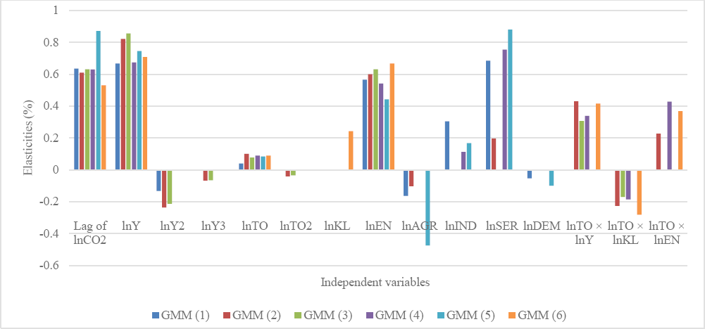
The estimated models in Table 1, produced parameter estimates that are in line with existing literature and support our theoretical expectations. However to check for the robustness of these findings we employed an alternative approach that is known for dynamic panel and able to control for potential endogeneity. This approach is known as GMM estimate. This is important because static RE models performed poorly and produce an inefficient estimate in the presence of endogeneity. Moreover, apart from the two different techniques of static and dynamic analysis we also check for the robustness of the empirical findings using linear and polynomial models with a different set of variables from the baseline model. Consistent with the static estimate, in dynamic GMM estimates our finding support most of our theoretical a priori with a little discrepancy in terms of parameter sign, magnitude, and statistical significance. This implies that our main conclusion and policy implications are not going to have any predicament.

Table 2 and Figure 2 reports the result of the two-step GMM estimate. We used the two-step because theoretically two-step estimator uses the best balancing matrices that are more efficient than the one step. From GMM estimates of Table 2, statistics from the test of second-order serial correlation of the disturbance and the Sargan and Hansen tests of over-identifying restriction, show that there is no second-order serial correlation, and our instruments set are also valid.

In Table 2, the coefficient of the lagged dependent variable in all specifications is positive and highly statistically significant. This implies that at any given period a change in any of the explanatory variables would significantly affect CO₂ emissions after the current period. This finding also supports the need to consider the dynamic model adjustment using the GMM approach because of the distinct short-run and long-run effects of the explanatory variables.

From the coefficient of the lagged dependent variable of the baseline model (1) in Table 2, the annual speed of adjustment which emissions can return to equilibrium in case of any deviation from the equilibrium level is 36% (1 – 0.639). With this low speed of adjustment, any deviation from the long-run equilibrium level of CO₂ emissions from the present period will require approximately three years to return to equilibrium. This result is supported by [1] and [20] who observed that current CO₂ emissions are influenced by the past emissions level in Sub-Saharan Africa.

Table 2

Dynamic GMM estimate for the effect of trade and energy on carbon emissions

	Polynomial models			Linear models
Model	(1)	(2)	(3)	(4)	(5)	(6)
Variables	GMM	GMM	GMM	GMM	GMM	GMM
Lag of lnCO2	0.636*** (0.111)	0.610*** (0.218)	0.631*** (0.173)	0.630*** (0.204)	0.871*** (0.268)	0.531** (0.219)
lnY	0.668** (0.292)	0.823** (0.324)	0.856*** (0.270)	0.674*** (0.200)	0.745*** (0.277)	0.708*** (0.240)
lnY2	-0.132** (0.0551)	-0.236* (0.130)	-0.213** (0.0987)	---	---	---
lnY3	-0.0217 (0.0281)	-0.0671* (0.0393)	-0.0655* (0.0350)	---	---	---
lnTO	0.0391* (0.0224)	0.100** (0.0470)	0.0780** (0.0384)	0.0889* (0.0504)	0.0834** (0.0368)	0.0890* (0.0508)
lnTO2	-0.00209 (0.0202)	-0.0415** (0.0196)	-0.0339** (0.0139)	---	---	---
lnKL	0.0519 (0.267)	0.0193 (0.150)	0.0802 (0.161)	0.0446 (0.149)	0.173 (0.530)	0.243* (0.127)
lnEN	0.566*** (0.172)	0.600*** (0.214)	0.631*** (0.190)	0.542*** (0.204)	0.443** (0.179)	0.667*** (0.213)
lnAGR	-0.164* (0.0892)	-0.103* (0.0586)	---	-0.152 (0.174)	-0.475** (0.216)	---
lnIND	0.305** (0.125)	0.0222 (0.0362)	---	0.113* (0.0671)	0.168* (0.0996)	---
lnSER	0.685** (0.289)	0.196* (0.102)	---	0.755* (0.424)	0.881** (0.434)	---
lnDEM	-0.0530* (0.0311)	-0.00441 (0.0509)	---	-0.0403 (0.0524)	-0.100* (0.0608)	---
lnTO × lnY	---	0.431*** (0.142)	0.307*** (0.0824)	0.339*** (0.129)	---	0.416*** (0.146)
lnTO × lnKL	---	-0.226*** (0.0824)	-0.171*** (0.0568)	-0.186** (0.0794)	---	-0.281*** (0.0993)
lnTO × lnEN		0.227** (0.111)	0.0715 (0.0628)	0.428** (0.180)		0.369*** (0.142)
Sargan test	42.61	30.92	47.48	34.26	34.17	39.12
Prob.-value	(0.122)	(0.320)	(0.078)	(0.314)	(0.364)	(0.251)
Hansen test	27.02	28.75	34.55	29.37	33.89	34.06
Prob.-value	(0.759)	(0.425)	(0.490)	(0.550)	(0.376)	(0.465)
AR(2)	0.58	1.37	1.15	0.42	0.11	0.40
Prob.-value	(0.560)	(0.171)	(0.250)	(0.672)	(0.915)	(0.687)
Observations	552	568	568	567	567	565
No. of group	47	47	47	47	47	47
No. of Instruments	47	47	47	45	44	45
Year Dummies	Yes	Yes	Yes	Yes	Yes	Yes

Note: Statistical significance of the estimates at less than 1%, 5%, and 10% are denoted by ***, **, and *, respectively. Robust standard errors are in parenthesis except for Sargan, Hansen, and AR(2) tests which are p-values.

Consistent with the RE model, in Table 2, GDP significantly increases CO₂ emissions. This further validates the scale effect and supports our theoretical a priori that increasing the scale of economic activities necessitated by trade openness increases CO₂ emissions. The baseline models (1) and (2) of Table 2 suggest that a 1% increase in GDP is associated with a 0.668% and 0.823% increase in CO₂ emissions.

The technique effect (Y²) significantly decreases CO₂ emissions and this is consistent with the random coefficient estimates of Table 1. The cubic component (GDP3) did not have the expected sign to validate the N-shaped nexus between GDP and CO₂ emissions in all estimates of Table 2. This further confirmed the EKC hypothesis and reject the N-shaped curve in the GDP and CO₂ emissions nexus.

The effect of trade openness (TO) is positive and significant in all the estimates. The baseline models (1) and (2) of Table 2 indicate that a 1% increase in trade openness increases emissions and degrades the environment by 0.0391% and 0.100% respectively. The squared of trade openness is negative and significant in models (2) and (3) of Table 2. This further provides evidence of a turning point in trade openness and CO₂ emissions nexus with an inverted U-shaped curve. This again supports the evidence that the pattern of the EKC is determined by the trade openness as obtained in the random estimates of Table 1.

The coefficient of the capital-labour ratio which measures the composition effect does not maintain its statistical significance in most GMM estimates of Table 2. This implies that there is no robust evidence that the composition effect increases CO₂ emissions after controlling for endogeneity. The little evidence of the composition effect observed in model (6) of Table 2 revealed that a 1% increase in capital relative to labour is associated with a 0.243% increase in carbon emissions and environmental degradation.

Consistent with the random coefficient, energy use positively increases CO₂ emissions and degrades the environment at a highly significant level of less than 1% in all the estimates. In Table 2 the elasticity of the energy effect lies between 0.443–0.667 suggesting that a 1% increase in energy use will result in between 0.443%-0.667% increase in CO₂ emissions and environmental degradation.

Using the dynamic GMM estimate the study further confirmed that African countries are having pollution from developed countries resulting from goods trade openness. The coefficient of the variable measuring this hypothesis is positive and statistically significant in all estimates (i.e. TO × Y > 0). This further validates the pollution haven hypothesis.

Consistent with a random coefficient of Table 1 the GMM estimate further confirmed that trade has allowed African countries to explore comparative advantage in labour-intensive export and production that are less polluting. This further confirmed the factor abundance effect/hypothesis because the coefficient of the variable measuring this hypothesis (TO × KL) is negative and statistically significant in all estimates of Table 2.

Similar to the static estimate, the GMM estimate also revealed that the net pollution haven effect is positive and harmful to the environment. This because the positive pollution haven effect (TO × Y) exceeds the negative factor abundance effect (TO × KL) in all estimates of models (2)–(4) and model (6) of Table 2. One possible reason for this positive net pollution haven effect is the African countries' level of development that is still within the phase of rising CO₂ emissions and environmental degradation.

After controlling for endogeneity the study further established evidence that the indirect effect of trade through energy is positive and harmful to the environment. This is because the coefficient of the variable measuring this effect (TO × EI) is positive and statistically significant in all estimates except in model (3) of Table 2.

So also agriculture value-added decreases CO₂ emissions and improves environmental quality. The baseline models (1), (2), and (5) of Table 2 suggest that a 1% increase in agriculture value-added is associated with 0.164%, 0.103%, and 0.475% decrease in CO₂ emissions and improved environmental quality.

Unlike in the random estimate of Table 1, in GMM estimate findings revealed that industry value-added degrade the environment by increasing CO₂ emissions. The estimate of models (1), (4), and (5) of Table 2 reports that a percentage increase in industry value-added is associated with between 0.113%–.0305% increase carbon emissions and environmental degradation.

Consistent with the random estimate the services value-added maintained a positive and significant effect on CO₂ emissions in all GMM estimates of Table 2. Therefore, in all the static and dynamic estimates, we established strong evidence that increasing the share of the services sector increases carbon emissions and environmental degradation in African countries. Finding from Table 2 revealed that a percentage increase in services value-added increases CO₂ emissions by 0.196%–0.881% respectively. This finding contradicts the theoretical a priori that increasing the share of services reduces carbon emissions and improves environmental quality.

Consistent with the static estimate, there is no strong evidence that a democratic government decreases CO₂ emissions and improves the environmental quality in African countries. In models (1) and (5) of Table 2 where democratic government assets a significant impact on carbon emissions, finding revealed that a 1% increase in a democratic government is associated with 0.0530% and 0.100% decrease in carbon emissions and environmental degradation.

In Figure 1 and Figure 2 we also presented the RE and GMM parameter estimates as presented in Table 1 and Table 2 to have a better look at the parameter stability and the effect of explanatory variables on the dependent variable. Figure 1 and Figure 2 only report the significant estimates because the insignificant estimates were not different from zero based on their statistical significance. In all the estimates there is a stable parameter estimate as indicated by different bars corresponding to each variable. In the random static estimate we established strong evidence of the scale effect (Y), technique effect (Y²), trade effect (TO), composition effect (KL), energy effect (EN), services sector value-added effect (SER), and pollution haven effect (TO × Y) on carbon emissions and environmental degradation. Except for the composition effect the strong effect of these variables has been further supported after controlling for endogeneity in GMM estimate as demonstrated by the bars corresponding to these variables in Figure 2. The factor abundance effect (TO × KL), trade and energy mediation effect (TO × EN), agriculture (AGR) and industry (IND) value-added effects, and the effect of democratic government were more strong and robust to linear and polynomial models in GMM estimate that control for potential endogeneity.

Figure 2

Parameters of dynamic models (Generalized method of moment)

This study used random coefficient and GMM estimate that is known for controlling endogeneity to a panel of 47 African countries and investigate the role of trade and energy in generating carbon emissions and environmental degradation. The empirical strategy revealed that the scale effect as measure by GDP increases emissions and environmental degradation. The technique effect decreases CO₂ emissions and improves environmental quality. These important findings confirmed the existence of the EKC hypothesis. Our finding rejects the existence of an N-shaped nexus between GDP and CO₂ emissions as confirmed by the coefficient of the GDP cubic component. Trade variable increases CO₂ emissions and degrade the environment, but there is evidence of threshold point at an advanced level of trade openness. This implies that at an advanced level of trade openness countries can have better access to environment-friendly technology that decreases CO₂ emissions and improve environmental quality. The Capital-labour ratio which measures the composition effect increases CO₂ emissions, this is more evidently observed using a random coefficient. The energy intensity is more CO₂ emission inducing based on its statistical significance and parameter magnitude. The empirical finding further confirmed both the income and factor endowment pollution haven in African countries. This implies that with goods trade openness the continent has gained a comparative advantage in both dirtier and cleaner export and production. This finding implies that, while trade openness is used by advanced countries to shift their pollution to African countries, it has also has allowed the continent to explore comparative advantage in clean labour-intensive export and production. We further observed that the net comparative advantage effect realized by African countries is positive and harmful to the environment. The indirect effect of trade through energy use has an increasing impact on CO₂ emissions and damages the environment.

The policy implications of these findings are that to mitigate emissions resulting from the increasing scale there is a need for the continent to improve on the technique of production and to reduce pressure on resource use in meeting both internal and external demand. This can be achieved by investing in areas of innovative technology that are more efficient and less polluting. The damaging effect of trade openness on the environment can be check if policymakers composed trade policies with environmental policies. This can be achieved by incorporating environmental policies into trade liberalization policies. To reduce the harmful effect of trade on the environment, there is also a need for the continent to eliminate or reduce trade barriers hindering the flow of technology that are environment-friendly. An international agreement is also required in addressing the challenges of rising CO₂ emissions. The result also revealed an important policy implication that trade may not necessarily have a direct beneficial impact on the environment by reducing CO₂ emissions but the impact can be indirect and mediated through input composition. To mitigate the rising CO₂ emissions resulting from energy usage there is a need for a steady transfer to renewable energy resources. This can be achieved by further exploring untapped renewable energy resources through investment. Since the price of renewable energy is comparatively higher, a policy aimed at targeting this can be more successful if it allows for wider access by making the price of renewable energy moderately lower through renewable energy consumption subsidies, lower import duties on solar panels and electric cars. TO prevent the further incidence of pollution haven in the continent strict environmental policies should be implemented, to penalized foreign affiliate companies and implement subsidy to encourage the use of energy-efficient equipment.