The importance of energy efficiency measures has been highlighted by the International Energy Agency (IEA) for achieving a low-carbon future and the potential for significant health and well-being. Nevertheless, the energy efficiency measures have a potential for negative impacts on indoor environmental quality (IEQ) if not applied and operated properly [1]. As the European and global community is threatened by climate change and the degradation of the environment, the growth of our communities should be approached in a sustainable way. The efficiency of resources and the sustainability of operating our buildings must be adapted to realise the environmental boost the world needs.

The Passive House building concept (also known under the German name Passivhaus), being highly energy-efficient, also highlights having a high level of IEQ, where the thermal comfort aspect forms a crucial part. Studies have been conducted to evaluate the thermal comfort status and other aspects through the post-occupancy evaluation (POE) processes. It is mandatory for the design stages, development, and certifications to go through the steady-state passive house planning package (PHPP), which does not provide a dynamic presentation of thermal comfort levels during the design stages.

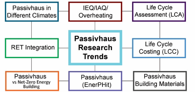
As the shadow of the climate change impact affects the building thermal status considerations, approaches are strongly recommended to be implemented for evaluating the building performance during the early design stages. Overheating percentages are rising each year, with global warming increasing the temperatures, pushing these percentages towards the PHPP standard top limit of 10% of the year’s hours, producing a performance gap later on. At the same time, no pre-realisation evaluation methods have been applied for future considerations, as Alhindawi and Jimenez-Bescos [2] presented in their study on this topic. As shown in Figure 1, research orientations related to Passive House vary according to aims and targets, whilst the main emphasis differs accordingly.

Figure 1

Passive House (Passivhaus) Research Trends in Literature

With higher insulation levels implemented in buildings for energy conservation, concerns regarding indoor air quality (IAQ) and ventilation adequacy indoors are increased, as higher levels of humidity. Overheating occurs due to such measures [3], especially while demands are expected to be increased in the foreseeable future under the impact of climate change [4].

In a study that looked into the IAQ status of a Passive House dwelling, Moreno-Rangel et al. [5] stated that certified Passive House dwellings are, in general, more efficient than conventional dwellings in many aspects. However, the occupant’s behaviour and the outdoor-sourced pollution play a significant role in how the building performs eventually.

Studies on energy efficiency and thermal comfort form a decent part of the Passive House research field, as in a study by Erba et al. [6]. They conducted a post-occupancy thermal comfort analysis of a certified Passive House in Sicily, Italy, taking the adaptive model as a base of investigation. Results showed that in summer, the passive techniques and features of the building had helped a remarkable performance to be achieved, especially with heat removal.

In another study taking the IEQ aspect as a base of research, Fletcher et al. [7] performed a temporal overheating evaluation, taking an empirical approach, in a certified Passive House building in the UK, which is living-assisted. Through monitoring for 21 months, in-use data were analysed to investigate overheating in the dwelling for the vulnerable occupants using the house by implementing statics and adaptive thermal comfort models, where this model related to naturally-ventilated spaces [8]. The results have revealed an apparent overheating during colder months whilst showing a substantial night-time overheating.

In a larger-scale investigation, Botti [9] conducted a POE study in a large Passive House-certified housing scheme in the UK, evaluating summer thermal comfort levels in the affordable housing development. A high overheating frequency was recorded through the analyses, which diverges from what the PHPP tool estimated. The study explained these results as due to multiple factors. The most important ones were the dense occupancy that caused higher internal gains than expected, as well as the usage of internal appliances accumulation, and in some cases, the insufficient reliance on natural ventilation to purge excess heat, led by the poor operability by occupants.

McGill et al. [10] presented a case study which included IAQ measurements, building surveys and occupants' diaries, on top of personal interviews with the occupants of a Passive House social housing project in Northern Ireland. The investigation results found issues with IAQ and the mechanical ventilation with heat recovery (MVHR) systems operation and maintenance. Another important finding is the occupants’ lack of knowledge and perception of overheating.

Sassi [11] examined the need for MVHR and natural ventilation in climates similar to the one in the southern areas of the UK. The study included thermal comfort, IAQ, and the energy impact of MVHR vs natural ventilation, through a POE study on two flats in Cardiff designed with the Passive House standards. Despite being a positive fact, the results found that energy consumption was significantly lower than the PHPP predicted, with no adverse effects on occupants' thermal comfort, IAQ. The study concluded that one could omit MVHR use without compromising thermal comfort levels and achieving low energy consumption, promoting the potential of a naturally-ventilated and ultra-low energy model.

The importance of the dynamic investigation of passive cooling effects on the thermal status of occupants, besides the thermal modelling prediction outputs, was also demonstrated by Olawale-Johnson et al. [12] while describing the variance in performance through implementing a combination of thermal modelling software. The authors stated that the dynamic simulation employment aided in acquiring reasonable predictions while comparing the results to the validation outputs of real-life monitoring data.

Zhao and Carter [13] researched perceived comfort in Passive House and expressed that the Passive House methodology leads to buildings with very high thermal efficiency and high levels of airtightness. Moreover, the focus of research on Passive House is mainly on energy performance, and the experience of occupying a Passive House is often overlooked. The authors considered social factors of comfort among Passive House occupants. The study compared the occupants’ expectations and perception of comfort, realising the approach by investigating the behavioural and psychological adaptive processes. The research focused on a range of Passive House developments built in the UK, studying them with the mixed-method approach. Findings showed a strong correlation between social aspects of comfort and participants’ evaluation of their building, stating that this association potentially reinforces the adaptive processes.

Alhindawi and Jimenez-Bescos [14] performed a comparative computational evaluation of thermal comfort levels in a pilot Passive House building in southeast England under the impact of climate change. The study implemented dynamic simulations and computational fluids dynamics (CFD) simulations, implementing the natural ventilation plan from the PHPP as a base of evaluation. Findings presented a set of predicted percentage of dissatisfied (PPD) values for different timeline-carbon dioxide (CO₂) emissions combinations, including recording a jump in PPD from 35% at the recent historical timeline of 2003−2017 to 94% at the timeline of 2080s of high CO₂ emission scenario proposed by the Intergovernmental Panel on Climate Change (IPCC), during summer peaks at each timeline. Results also identified a set of descriptive outputs regarding psychrometry, thermal sensation, and effective temperatures, clarifying the positive impact of dynamic simulations on the Passive House thermal comfort levels prediction scale.

In their research that looked into assessing sustainable buildings, Tagliabue et al. [15] demonstrated the importance of dynamic outputs for building assessment and evaluation. Although the research focused on post-realisation building monitoring, the results showed the dynamic variation in thermal comfort and IAQ conditions during different occupancy/usability patterns, supporting the need for pre-realisation dynamic evaluation of the IEQ aspects.

Another computational study by Dodoo [16] looked into the status of thermal comfort in buildings in a predictive approach in Sweden under the impact of climate change. Simulations predicted a 33% increase in PPD, in parallel to a 3 °C increase in indoor air temperatures by 2050.

The accuracy of computational studies predicted mean vote (PMV)-PPD results is a significant factor one must consider when conducting simulation studies. At the same time, validation and calibration are crucial before adapting prediction models. Cheung et al. [17] referred to that matter in their study of the PMV-PPD accuracy. They noted that the accuracy of PMV prediction of thermal sensation is around 34%, as of three times observations/calculations, only one is correctly predicted. Additionally, results stated that the PPD approximation was 15−25% overestimated.

Charai et al. [18] involved a calibrated PMV-PPD model in their study of thermal comfort in buildings. The study emphasised the importance of calibrating thermal comfort models and supported that by implementing a validated PMV-PPD model in EnergyPlus. Results presented a PPD of 54.5%, which was similar to the simulated one (54.6%).

Gilani et al. [19] investigated thermal comfort levels in natural-ventilated residential buildings. The study noted the importance of accounting for over-estimation and under-estimation of the PMV equation application in summer and winter. The results showed a 13% underestimation of thermal sensation in summer and 35% overestimation in winter.

A study by Parker et al. [20] described the use of calibrated dynamic thermal simulation models of an as-built certified Passive House dwelling. The researchers aimed to evaluate the potential for natural ventilation to avoid excessive summertime overheating. The study evaluated the impact of user-controlled natural ventilation on regulating internal summer temperatures. Absolute and adaptive thermal comfort metrics were implemented to predict future overheating levels in the Passive House. The results suggested that the extended periods of window opening can help avoid overheating in this type of dwelling. This is realistic under both current and future climatic conditions.

As shown in a chosen range of literature, studies implemented various approaches and mechanisms of research to be integrated with the Passive House building concept and its performance aspects, with a special field that takes thermal comfort as a main base of investigation. It still is not adequately investigated in an acceptable way that implements the dynamic parameterisation of inputs, especially in a predictive process during the early design stages. The previous facts have formed a knowledge gap in this field of study’s literature, while the imbalance existed between early design stages and POE results.

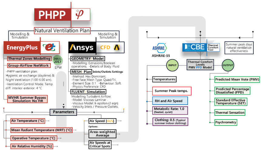
This paper presents a methodological approach which aims to create a comparative evaluation of thermal comfort levels in a pilot Passive House simulation project based on the PHPP natural ventilation plans. The implementation of other pieces of software with a dynamic simulation nature enables gaining a predictive image of the thermal comfort status of the indoor space during the pre-realisation stages.

The methodological approach suggested in this work takes the PHPP as a base for data extraction in a two-stage modelling process of a pilot Passive House in a simulation project in Chelmsford, England, UK.

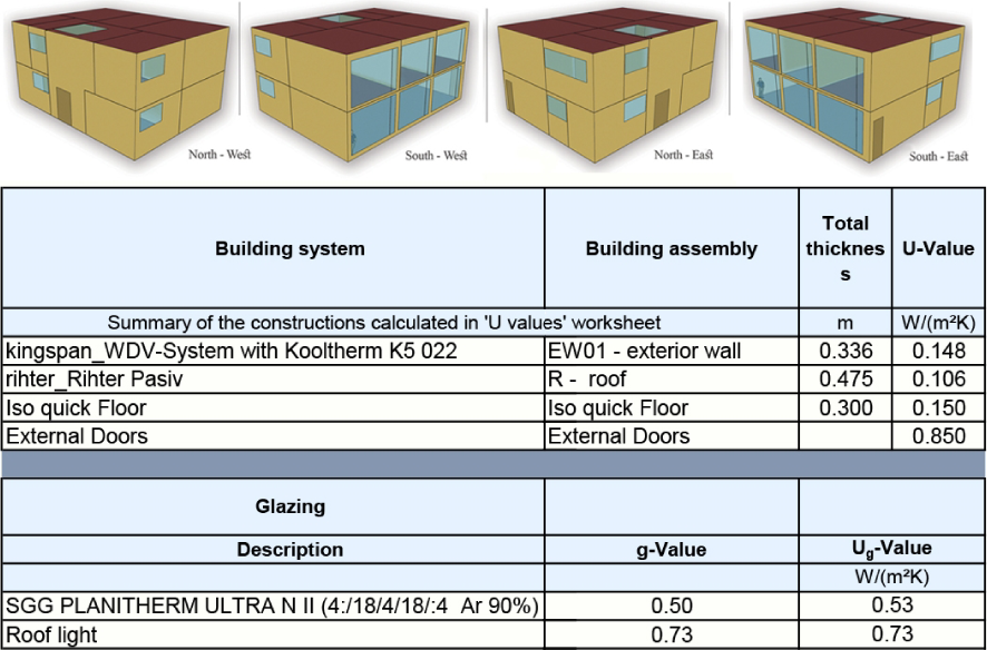
The first stage comprises the thermal modelling of the Passive House dwelling in EnergyPlus, to extract the Passive House construction data from the PHPP and apply the information in the EnergyPlus simulation setup. This step was done through SketchUp Make software for modelling, with the Euclid Plugin connecting it to EnergyPlus (EP).

The objective of the first stage was to produce the parameters that are related to thermal comfort calculations, such as air temperature (T_a), operative temperature (T_o), mean radiant temperature (MRT), and relative humidity (RH). The MVHR system’s summer bypass mode was simulated during the setup, which works as an air exchanger with no heat recovery in the process while activated in summer. Figure 2 presents the EP Model and the construction data applied from PHPP.

Figure 2

EP Model - PHPP Construction Details Extracts

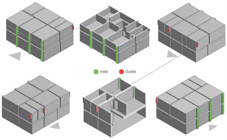
The second stage comprises the employment of CFD modelling and simulations through ANSYS software. The first part of the second stage included applying the Passive House dwelling’s physical properties for modelling in ANSYS GEOMETRY. By translating the PHPP natural ventilation plans (Hygienic and Night Ventilation) through the windows opening dimensions and areas, air inlets and air outlets were identified in ANSYS MESH, according to the prevailing wind direction of the site.

The final part of the second stage was done through ANSYS FLUENT, where the simulations were performed for the modelled Passive House to extract air speeds in a detailed report of the indoor spaces of the dwelling. The outputs also have the option to extract air speeds at specific points in the indoor space or air speeds as area-weighted averages (A-WA) of each room.

Figure 3 illustrates the ANSYS model. The suggested inlet airspeeds of test were 0.5 (low), 1.0 (medium), 1.5 (high), and 2.0 (very high) m/s. The objective of this stage was to obtain air speeds required in the thermal comfort calculation stage as a main influencing parameter. The employment of these specific inlet air speeds in the FLUENT settings came from applying several site-specific wind speed analysis steps.

The general pattern is that wind speeds tend to be lower in urban areas than in surrounding open/rural areas (where the weather stations usually are) because of the friction forces of the urban texture/building surfaces.

Figure 3

ANSYS CFD Model

The vast majority of weather stations for wind speed measurement are positioned in open areas like airports (e.g., the weather database source of this work). This may lead to overestimating the wind speed values outputted by simulation results, leading to an inaccurate estimation of the ambient wind effect on building natural ventilation effectiveness and performance.

The frictional drag creates a slowing effect on wind speeds while wind travels within the urban areas; therefore, the wind speed data obtained from the simulations EP weather data file (EPW) were analysed to acquire a more accurate set of wind speed values for utilising as inlet air speeds in CFD simulations.

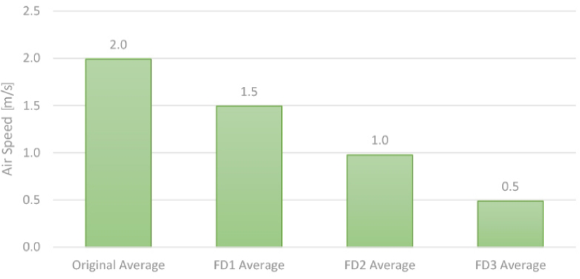
Eventually, they produced the indoor air speeds used in the thermal comfort calculations. The method applied suggests the friction drag decreases the airspeeds by 30−50% as a minus multiplier [21]−[24]. Figure 4 shows the diminishing effect post-application on a monthly peak day basis, while Figure 5 shows the averaged airspeeds during summer, with the friction drag effect.

Figure 4

Drag Effect on Wind Speeds − Peak Days

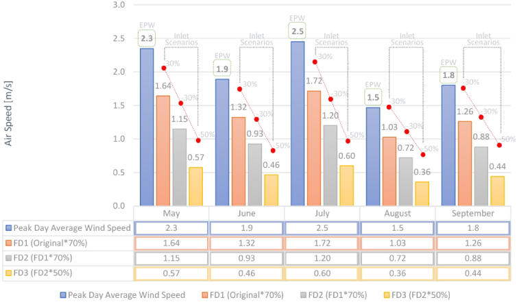
It may be clarifying to mention that the inlet airspeeds suggested are responding, not to multiple weather data wind velocities, but to the summer peak days’ daily average value of wind that happens to be at that day (a peak day of each summer month), taken from the weather file. Consequently, the inlet airspeeds suggested are produced from this specific daily average of 24 hours, which is then affected by the friction drag (FD) effect in one to several (in our case, three) minus multiplications. Hence the presented FD1, FD2, and FD3 represent inlet speeds at three scenarios, responding to three levels of friction drag that are simulated in this process.

Figure 5

Drag Effect on Wind Speeds − Summer-Averaged

A previous study that has purely focused on the CFD modelling and simulation of the case study Passive House of this research has more details. These include the ventilation plan application, airflow patterns, critical interior space analysis, and a comprehensive description of the airflow performance at specific airspeeds and positions [25].

Stage three, which realises the main objective of this study, comprises calculating thermal comfort levels in the Passive House according to the parameters extracted from the previous two stages of EnergyPlus and ANSYS CFD simulations.

The thermal comfort levels were calculated by employing The Centre for the Built Environment (CBE) Thermal Comfort Tool [26], [27]. It is a free and robust online tool for thermal comfort calculations and visualizations that complies with the American Society of Heating, Refrigerating and Air-Conditioning Engineers (ASHRAE) 55-2017 standard of Thermal Environmental Conditions for Human Occupancy [8]. The tool offers a range of describing features of the thermal comfort status. The demonstration examples of this methodology application have been selected for summer peaks extracted from the simulation EPW file in EnergyPlus.

The timeline of the weather file takes the weather status of the period from 2003 to 2017 (TMYx.2003-2017), exported from OneBuilding organisation [28], a repository of free climate data for building performance simulation from the Creators of the EPW.

TMYx files are typical meteorological files derived from ISD (Integrated Surface Database) with hourly data, using the TMY/ISO 15927-4:2005 methodologies [29]. These years’ weather parameters are a representation of the historical range. Of course, this methodology could be applied using any weather file representing the simulator's targeted timeline/year. The weather data repositories for building simulations EPW files do not necessarily mention the nature of construction in a detailed description, rather than mentioning that the EPW file (TMYx.2003-2017.epw is our case) data are derived from the most recent 15 years (2003−2017).

Our approach included averaging, which had been done on the 24-h scale regarding wind to simulate scenarios, but not for temperatures and RH values. These already are representatives of the whole timeline more than being considered average. However, the peaks might not be as severe as some timeline year’s if a specific year’s EPW file was selected for simulation.

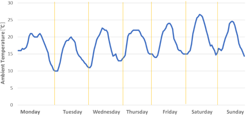
The summer peaks are represented by the peak of each month of the summer months; May, June, July, August, and September [30], for which the hourly-basis temperatures and RH values were extracted. An important matter is that the UK climate could provide a sufficient diurnal temperature swing, even during summer temperature peak days. The ambient temperature patterns shown in Figure 6 illustrate the design week in the example summer month of August. This means that the day-night temperature difference will lead to the night flush ventilation, potentially reducing the hours of overheating during the day by precooling the indoor spaces during the night, allowing radiant cooling to occur during the day.

Figure 6

Summer Design Week (August) − Diurnal Swing

The ANSI/ASHRAE-55-2017 standard notes that the adaptive method is used for thermal comfort status evaluation for naturally-ventilated spaces. The empirical model associates the environmental measurements to the occupant's satisfaction, while the prevailing mean ambient air temperature determines the position of per cent satisfied contours bordering the comfort zone. Although this research presents thermal comfort evaluations based on natural ventilation, the PMV-PPD method is implemented. The simulations propose that the MVHR summer bypass is on besides the natural ventilation plan (considered as hybrid ventilation).

Temperatures extracted from the EnergyPlus simulations represent the effect of both natural ventilation being operated and the summer bypass mode being activated. Therefore, the CFD simulations follow to evaluate the airflow patterns and the indoor air velocities that happen to occur while ventilation is on.

The environmental measurements in the PMV method are incorporated with assumptions about the level of clothing (assumed as 0.5 for typical summer indoor clothing) and the activity level or the metabolic rate (assumed as 1 for a seated, quiet person) for calculating PMV.

The previous inputs represent a measure of an average occupant’s thermal sensation. The diagram in Figure 7 explains the workflow, presenting some basic settings for the Passive House modelling in EnergyPlus and ANSYS.

Figure 7

Workflow Diagram

Other parameters that were accounted for in EnergyPlus include the modification of some dynamic classes in EnergyPlus simulation settings, including:

• Class: Building

• Object:

• - Terrain: Suburbs,

• - Loads Convergence Tolerance Value: 0.04,

• - Solar Distribution: Full Interior and Exterior,

• - Warmup Days Range (min−max): 6−25.

Results are presented for each modelling stage separately, characterised as the thermal modelling stage (EnergyPlus), computational fluid dynamics stage (ANSYS), and thermal comfort calculations stage (CBE Tool).

Computational fluid dynamics modelling stage

The natural ventilation plan drawn from the PHPP and applied for investigation in the ANSYS CFD simulations was tested for three inlet air speeds (low, medium, high), which are usually coming in from the windows of the building at the site. Figure 3 earlier shows the simulated model. Figure 8 shows details of the simulated areas.

Figure 8

CFD Simulation and Simulated Spaces

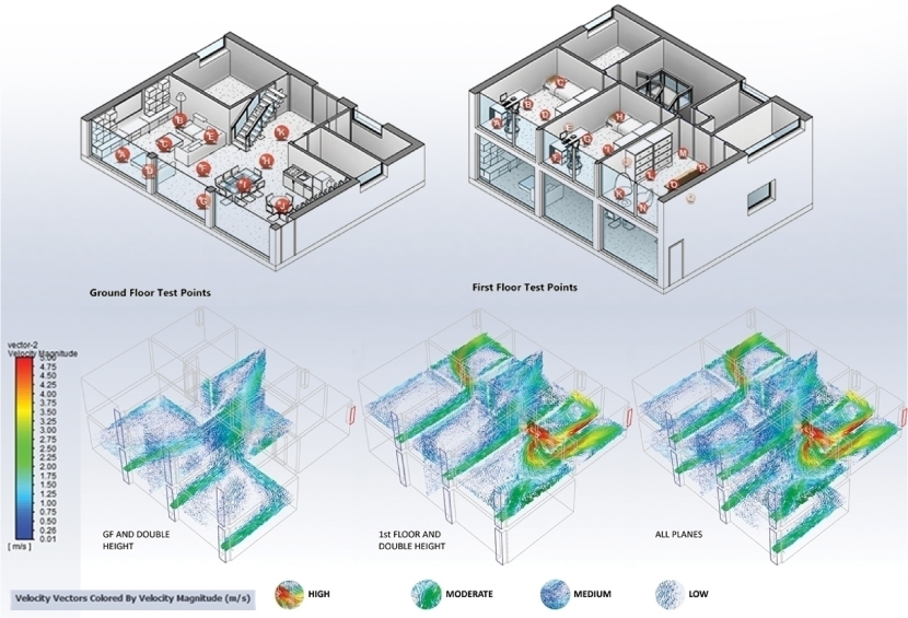
The test considered two approaches for extracting air speeds in the indoor space. Therefore, two sets of air speeds were produced: air speeds at multiple points that cover the simulated areas and the area-weighted average air speeds that represent the average air velocity of the whole simulated room space.

Three representative area-weighted average indoor air speeds were extracted from the simulated areas of the Passive House for use in the thermal comfort calculations later. The lowest speed was 0.19 m/s, medium AW-A 0.58 m/s, and high AW-A 1.17 m/s, after simulating the previously mentioned assumed inlet air speeds from the ambient (the friction drag assumption), drawn from the weather file data.

For modelling simplicity, aiming to demonstrate the method, the three air speeds were used in the next calculations. It was not assumed that these are continuously produced in the indoor space but are taken as values that may represent an averaged extent describing the existing airflow pattern.

CFD simulations of the model also provided a sufficient description of the airflow patterns through the ANSYS FLUENT “surface integral reports”. These produced a comprehensive interpretation of how the PHPP natural ventilation plan works within the Passive House spaces. The air velocity values stream through the inlets and outlets while considering the inlets as “velocity inlets” and the outlets as “pressure outlets”.

Figure 9

A-WA and UI Correlations

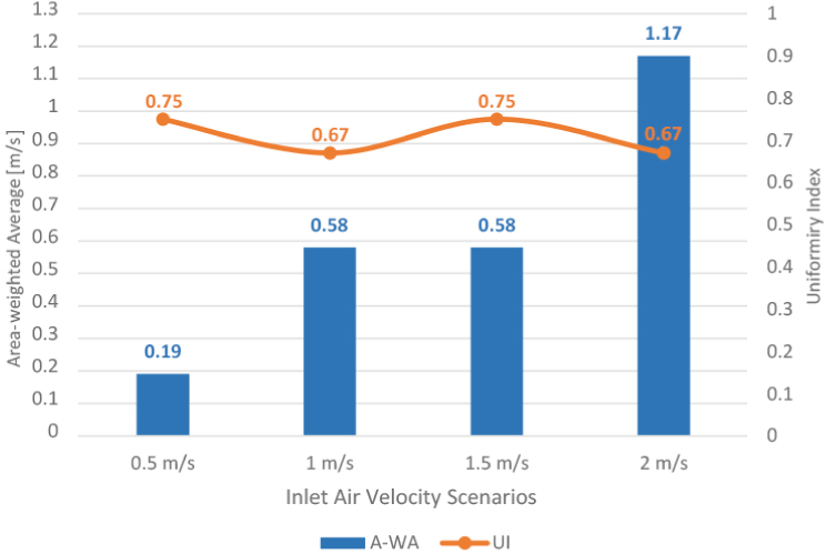
Additionally, and as Figure 9 shows, a description of the Uniformity Index (UI) could also be implemented to evaluate this methodology. UI ranging from 0 to 1 describes how uniform the air distribution is throughout the areas of the simulated space; the higher the UI value, the better the air distribution is in the simulated space.

Although the next example’s values are purely hypothetical, 0% has no uniform distribution, and 100% has fully-uniformed air distribution. This provides another balance aspect to the natural ventilation planning and thermal comfort investigation through the design stages. In Figure 9, the lower/higher inlet air velocities do not necessarily lead to a higher UI. Nevertheless, these inlet air speeds are tested to be controlled by the natural ventilation plan operation, while the windows opening areas and the air stream direction balance, with the outdoor air characteristics playing a major role.

The combination of modelling in EnergyPlus and ANSYS CFD in the two previous steps has provided the required parameters that will be implemented in thermal comfort calculations in the next step. Dynamic production of these parameters is shown, thus leading to flexible calculations results of thermal comfort levels, to be predicted in early design stages. While presenting a dynamic description of the airflow pattern, sustainable advantages are realised through this workflow step by supporting sustainable design targets of ventilation and air distribution aspects of practicality.

Thermal comfort calculations stage

The CBE Thermal Comfort Tool has many features to present results with while offering various outputs that help describe thermal comfort levels. In PHPP, a limited description of thermal comfort is offered, with no estimation by calculating the PMV-PPD or any investigation opportunities to employ the variance of thermal comfort parameters in different situations.

To avoid any confusion regarding the PPD percentage limit, above which the rates are considered uncompliant, some explanation may clarify the PPD results threshold of evaluation followed in this work’s results. Implementing the ASHRAE standard 55, the definition of the comfort zone comes as conditions including PMV levels from −0.5 PMV to +0.5 PMV, where the occupants’ percentage of dissatisfaction is predicted through the PMV curve. With the PMV empirical profit fit of the thermal sensation method, a PMV of ±0.5 predicts 90% of a population satisfied, or a 10% PPD.

Nevertheless, this 90% satisfied occupants rate is rarely obtained, with around 80% of maximum satisfaction. The widely-spread misunderstanding of this PPD rate is usually considered 20% maximum. The difference has been credited to the discomfort in local parts of the body perceived by occupants. The prediction of local discomfort probability is realised by testing environmental parameters measured in sensitive locations against the limits determined empirically.

The effects of local discomfort are assumed to contribute an additional 10% of PPD to the discomfort predicted by PMV. Hence the expected total PPD in a building, with PMV ±0.5, will be 20%. Nevertheless, the CBE Thermal Comfort Tool employed in this methodology considers the 10% PPD threshold, excluding the local discomfort, and not the combined 20% occupant satisfaction evaluation that other tools have in general, following standard 55. As described in Figure 9 earlier, the outputs form a comprehensive prediction of the comfort status of the occupants.

Starting with PMV, Figure 10 shows the PMV values during the night ventilation operation. It explains how the thermal sensation levels are out of comfort range for being cool, even at a summer peak day, due to the day-night temperature high difference, and slightly cool according to the thermal sensation index, referring to how night ventilation could participate in cooling the indoor space through night flush, decreasing the higher indoor space temperatures at daytime.

Figure 10

PMV Values Comparison − Night Ventilation

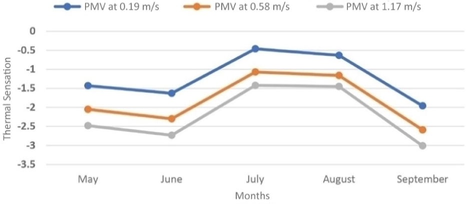
The comfort levels are estimated to be easily retrieved by the occupants at night. They are adaptive to the cool status by adjusting their clothing level (levels in the calculations were fixed at “typical summer clothing”) and bed covers.

Temperatures averaged for the timeline of simulations EPW has surely lessened summer peaks' severity. Nevertheless, the results have gone the other way, as the thermal sensation levels were recorded in the cool range instead of being in the warm range, which is the supposed case where temperatures reach around 30 °C during mid-day. However, the main purpose of this process is to apply the methodology, more than giving verdicts on the impact of data averaging or how variant the EPW data could be, affecting the results in one way or another, although this may also be considered as an outcome of the study.

An important point to highlight is the negative values (referring to occupants' cold sensation) of PMV recorded. For all thermal comfort reporting, though the produced values for thermal comfort “vote” have a discrete scale (e.g., –3 to +3 or –4 to +4), the calculations are carried out on a continuous scale and, thus, reporting may be “off the scale” with specific conditions encountered in the space. This is not necessarily an error in reporting; rather than a different approach that does not consider the “limits” of the discrete scale values. So, suppose the model has a combination of thermal comfort parameters that would make occupants very cold (low clothing level, high airflow/draught, etc.). In that case, theoretically, negative PMV values could be achieved. Practically, the aim is to keep PMV values as close to 0 as possible to maximise occupant thermal comfort.

As shown in Figure 11, the presented area-weighted averages of the airflow pattern of simulation have produced a range of PPD values, where the majority of the summer months’ peaks PPD values were not compliant with the ASHRAE-55 standard. Despite the results corresponding to higher temperatures, the planned ventilation rate may lead to dissatisfaction with thermal comfort, referring to the fact that less ventilation is required or a modification of the ventilation plan is needed (i.e., window opening area, time, duration, airflow control). While only the 10% PPD of the July peak, at 0.19 m/s, was compliant with the ASHRAE-55 standard, all the other Summer monthly peaks' PPD rates recorded a gradual increase in percentage, in parallel to the increase of the air speed tested in calculations.

Figure 11

PPD Rates Comparison

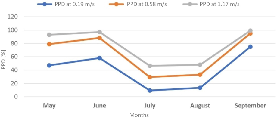
The only compliant PPD rate was calculated for July T_o peak, during the 0.19 m/s A-WA test, with the closest rate in August T_o peak being uncompliant, with 13.3%. As shown in Figure 11, the other parameter combinations calculated by the tool were not successful in producing compliant PPD rates. The percentages reached as high as 97.1% in June, and 99.2% in September, for the A-WA of 1.17 m/s (produced from the very high inlet air velocity), while the medium A-WA air speed of 0.58 m/s, PPD rates were, as well, higher than being compliant with the standard.

While presenting all these PPD values, it is important to reiterate the need for accuracy considerations regarding simulation results, for PMV-PPD in specific, as noted earlier in literature [17]. Furthermore, the results also provided other descriptions for the ventilation status effect, represented by the cooling effect ranges for the tested thermal comfort parameters, as shown in Figure 12.

Figure 12

Cooling Effect Comparison

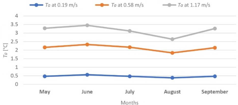
The cooling effect varied while the indoor A-WA air speed changed, recording lower rates with lower air speeds as the cooling effect rotates around 0.5 °C. In addition, the cooling effect multiplies with the increasing air speed, going above 2 °C as recorded in all summer months during the 0.58 m/s test. The cooling effect reached 3.45 °C as recorded in June, while the A-WA air speed test was 1.17 m/s.

Results from the CBE Tool provided a sufficient representation of other aspects of describing the thermal comfort status, including psychrometric charts, parameters correlations, and outputs charts. All the previous outputs made it flexible for the simulator to investigate the design performance in a predictive process while making available comparisons of different thermal comfort parameter combinations.

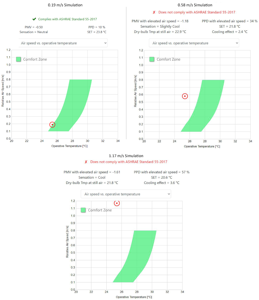
Figure 13 shows the results of the calculation runs for the July T_o peak hour at 0.19 m/s, 0.58 m/s, and 1.17 m/s. The charts illustrate the correlation between relative air speed within the space and the operative temperature, showing how the uncompliant parameter combinations perform under the shown outputs. At the same time, the red dots represent the in/out of comfort range of the performance. Whereas the 0.19 m/s simulation is at the edge of the comfort zone, compliant with 10% PPD, the other two simulated airspeeds, 0.58 m/s and 1.17 m/s, outputted incompliant PPD values of 34% and 57%, respectively.

Figure 13

T_o vs. Relative Air Speed, July Peak Day simulation − CBE Tool Chart

Another representation of results for the previous examples’ similar simulation boundaries is visible in Figure 14. It draws the traditional psychrometric chart of the operative temperature vs humidity ratio while producing a set of outputs describing the thermal comfort status of the indoor space for the parameters combinations.

The investigation of the night ventilation plan derived from the results shows a high potential of reducing temperatures overnight to keep the temperatures low during the day. At the same time, in more common spaces (living, dining, and corridors), thermal comfort tends to fall within the cool thermal sensation status, with a cooling effect of above 2 °C. On the other hand, bedrooms may have another thermal sensation status while the doors are closed at night, with the occupants’ individual preference to operate the room’s window.

Figure 14

T_o Psychrometric Chart, July Peak Day simulation − CBE Tool Chart

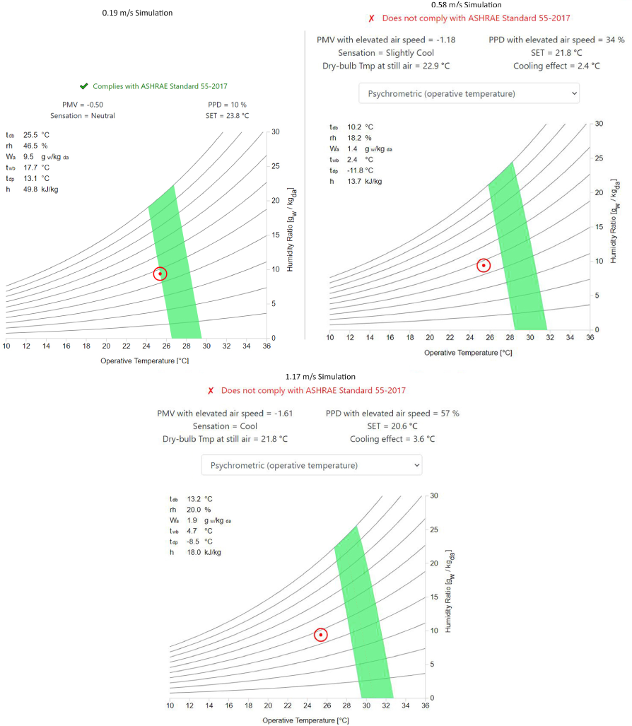
With an operative temperature of 25.3 °C occurs, the calculations show that the standard effective temperature is 21.8 °C, being set between a dry bulb temperature of 22.9 °C on the other side; hence the cooling effect is being subtracted from the operative temperature, only to produce the standard effective temperature. These test calculations could relatively easily control that during the early design stages to push the ventilation plan towards a more efficient performance and further robust temperature control, then eventually, a more accurate prediction process. This may balance the PMV value within the thermal sensation index of the occupants, targeting the position closer to the comfort zone conditions, including PMV levels from −0.5 PMV to +0.5 PMV. In the psychrometric chart in Figure 14, the abscissa is the operative temperature, and for each point, the dry-bulb temperature equals the mean radiant temperature (DBT = MRT).

Additionally, Figure 15 shows how some variables, calculated using the standard effective temperature (SET) model, vary as a function of the input parameters of thermal comfort calculations. The results example shown are for the area-weighted averages of 0.19 m/s, 0.58 m/s, and 1.17 m/s calculation runs for the July temperature peak hour.

Figure 15

SET Outputs, Results Example − July Peak Day

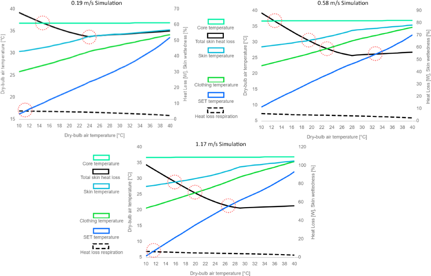
The charts in Figure 15 show how designers could leverage the included information with further details during the design stage investigations of performance and describe the thermal comfort variables between DBT and heat loss with skin wetness. The visualisations represented by the SET model show the relation between the skin temperature, mean body temperature, core temperature, clothing temperature, and other aspects of sweat-evaporation induced skin heat loss and sensible heat loss, with totals of the heat loss coefficients of the mentioned aspects. While these aspects are important considerations for thermal comfort details of the occupants, the model shows how lines form cross points that lead to the description, derived from the parameters combination inputted originally. In addition, it is shown how these cross points are being shifted in parallel to the change in air speeds alone, giving a flexible and complex output possibility for designers to balance other parameters altogether, aiming at reaching a stabilised performance prediction. In parallel to dynamic outputs, the process of such investigations may add a concentrative status explanation of the mentioned aspects, aiding designers significantly in acquiring an idea of how these parameters are affected in correlation to the dynamic status of thermal simulation outputs.