


Activities like Hospitals or Healthcare Facilities are often characterised by peculiar energy requirements. Indeed, they must be in operation continuously during the day, every day of the year [1]. Furthermore, healthcare buildings need several energy vectors to ensure the continuity and efficiency of energy systems and various medical services. A survey of the thermal and electrical energy needs in several private hospital buildings in Spain, covering the period from 2008 to 2017, was conducted to assess their main energy drivers [2]. Correlation analyses were carried out between the energy requirements of the buildings and several features. The outcomes highlight that energy consumption strongly correlates with the useful floor area. Contrarily, a weak correlation has been found with other activity parameters like the staff on duty or the number of inpatient rooms. Furthermore, the specific constraints of indoor air quality [3] lead to sophisticated Heating, Ventilation and Air-Conditioning (HVAC) systems to meet security and comfort standards [4]. These systems require electricity to fulfil the ventilation requirements and thermal energy (e.g., hot water, chilled water and steam) for air handling. Furthermore, refrigeration systems are typically a significant contributor to the increase in energy demand [5]. Chillers typically require cooling towers for their functioning, leading to a further increase in water and electrical energy consumption. Since HVAC systems are among the main energy-intensive applications of a healthcare building, external climate conditions like outdoor air temperature or humidity might be key energy drivers.
Hu et al. [6] report the electricity consumption of a large acute hospital in Taipei City (Taiwan), highlighting the major influence of the chillers on the overall building electricity consumption. Renedo et al. [7] analyse different possibilities for providing heating, air conditioning and hot tap water to a hospital centre, showing the high electricity consumption for air conditioning purposes, especially during the summer. Congradac et al. [8] developed a mathematical tool to calculate room/building energy demands. Preliminarily, the paper analyses the energy balance of a hospital facility, highlighting that heating and cooling energy demand represents 48% of the overall energy consumption of the building.
Twenty hospitals were analysed between 2005 and 2014 to highlight correlations between building energy demand, outdoor climatic conditions, and building envelope characteristics [9]. Results show a significant correlation between the outdoor air temperature and the building energy demand. Furthermore, several studies were conducted to assess the impact climate change has on building energy consumption, focusing on indoor climate control applications in the healthcare sector, confirming a strong hospital energy demand dependency on climate parameters. Nematchoua et al. [10] analyse the impact of climate change on the heating and cooling energy demands in several hospitals on six islands in the Indian Ocean. Lomas and Giridharan try to find several retrofit measures to maintain internal thermal comfort standards and thermal resilience to climate change of Addenbrooke's Hospital [11] and Bradford Royal Infirmary [12] in the UK.
The air handling systems often markedly influence the overall hospital energy demand. Nevertheless, the healthcare core activities can play a relevant role in shaping energy demand, depending on the specific activities carried out within the facilities. A study by Rohde and Martinez [13] aims to analyse the energy consumption related to the medical equipment of a large Norwegian teaching hospital. The analysis results report a daytime electricity consumption of about 90 kWh/m2 per year. Christiansen et al. [14] analyse the electrical energy consumption related to the medical equipment of hospital laboratories, evaluating their impact on the overall energy demand during healthcare facilities' operation.
Compared to other activities and buildings, healthcare buildings and hospitals present specific energy demands. Eckelman and Sherman [15] found that hospitals and healthcare facilities in the U.S. are among the most energy-intensive commercial buildings. Indeed, they present high energy consumption per square metre, doubling that found for a standard office building. The energy inefficiencies of healthcare facilities can be related to a non-optimised HVAC systems management strategy. Consequently, developing energy-saving strategies to improve the performance of HVAC systems could lead to important energy savings. El-Baky et al. analyse the effectiveness of heat pipe heat exchangers to perform heat recovery in air conditioning systems and improve their energy efficiency [16]. Cuce et al. [17] analyse several solutions to monitor and improve the internal climate of a residential building. Moreover, Fernandez-Seara et al. [18] conduct an experimental analysis of air-to-air heat recovery units for residential building ventilation purposes, investigating their performance by varying the operative conditions.
The energy performance of buildings can be improved by implementing optimal management strategies through dedicated Building Energy Management Systems (BEMS) [19]. Jafarinejad et al. [20] propose a bi-level energy-efficient occupancy profile optimisation method integrated with a demand-driven control strategy adjusted with dynamic set-point temperature to optimise the system control strategy of a University building. Moreover, Mauri et al. [21] study low-impact energy-saving strategies for heating systems of modern residential buildings in Rome (Italy).
Nevertheless, the development of an energy-saving strategy must involve detailed analyses and characterisation of the energy needs of the specific activities. Consequently, it is essential to carry out studies to define the parameters that mainly influence the building energy demand. In other words, one must develop an effective energy-saving strategy according to the behaviour of the main energy drivers.
Several numerical techniques have been exploited to perform statistical analysis on building energy consumption to identify the energy drivers of different buildings typology. Ürge-Vorsatz et al. [22] analyse the energy drivers related to thermal energy needs on a global and regional basis, investigating their trends in the next future. Wang et al. [23] analyse the energy consumption of public hospitals in China, obtaining valuable information about the energy drivers. Li et al. [24] studied the influence of climate, building size, and building technologies on building energy performance, highlighting that although all are important, none are decisive factors in building energy use.
Several modelling tools have been studied to investigate buildings and their energy systems better. Harish et al. [25] and Subramanian et al. [26] review several simulation methods and tools that can be useful to model building energy systems. As specific energy requirements can characterise a healthcare facility, energy drivers are the key to better understanding the test cases under analysis. Moreover, one must assess the application of energy-saving strategies through further analysis of the building energy consumption. Consequently, numerical modelling of the building energy demand based on the already defined energy drivers is essential.
The literature recognises regression analysis as a viable way to monitor the evolution of energy drivers, using [27] to carry out electrical and thermal load forecasting. Aydinalp-Koksal and Ismet Ugursal [28] compare the artificial neural network regression methods to several engineering approaches for building energy consumption modelling. The regression technique uses multiple linear regression analysis to determine the coefficients of the model corresponding to the selected input parameters, providing an equation able to quantify the building energy demand based on these parameters [29]. Braun et al. [30] exploit multiple regression analysis as an energy forecasting tool for a supermarket in Northern England in the period 2030−2059. They use gas and electricity data for 2012, using external air temperature and relative humidity as energy drivers.
Moreover, various advanced machine learning techniques enable effective models for building energy forecasting purposes [31]. The Artificial Neural Network models represent an example. In particular, Ilbeigi et al. [32] perform energy prediction and optimisation for an office building through artificial neural networks and genetic algorithms. On the other hand, Buratti et al. [33] carry out residential building behaviour simulations using Artificial Neural Networks, using several different features like climate conditions and thermal characteristics of building envelopes as input parameters, aiming to predict the indoor air temperature.
If more detailed information about the analysed structure is available, the Building Energy Modelling technique (BEM) represents a viable way to simulate the building energy requirements behaviour. Booten et al. [34] use a dynamic building energy simulation software (EnergyPlus) to study the effectiveness of advanced cooling strategies in residential buildings. Gesteira et al. [35] exploit TRNSYS software to estimate the heating and cooling energy demand of a single-family dwelling.
The discussed numerical models can be used to realise tools aimed at monitoring the building energy consumption behaviour. In particular, the energy consumption model can be used as a standard building energy demand to compare future energy consumption with the standard ones. This comparison can be useful in detecting abnormal behaviour in energy use, making it possible to identify malfunctions in the management and operation of the equipment and systems installed in the facility. A widely used method consists of the realisation of a statistical process control chart called CUmulative SUM of differences (CUSUM) [36]. Fichera et al. [37] use the CUSUM method to carry out energy performance monitoring of several buildings of public organisations.
In a previous study carried out by the authors on a healthcare facility located near Florence (Italy) [38], an analysis of the 2019 building electricity consumption was conducted. The aim of the present work is to extend the previous analysis by introducing new data about energy consumption and exploiting the data to realise an offline monitoring method based on the CUSUM technique.
Although similar approaches can be found in literature, it is difficult to find studies on peculiar applications like hospitals and healthcare facilities, where the amount of available data allows an in-depth analysis of the electricity demand and a correlation study involving internal and external features. Moreover, the study explores the possibility of manipulating available data to maximise the model prediction capabilities. More advanced techniques such as Artificial Neural Networks can be exploited to carry out energy predictions. Despite the generally better performance of such techniques, their complexity leads to losing consciousness of the data elaboration process. Moreover, more complex and advanced methods require a greater computational effort, not only for the training procedure itself but also for the fine-tuning procedures necessary to check the validity and generality of the model. Consequently, carrying out a preliminary study of the problem using simple models makes it possible to obtain a better knowledge of the system studied from an engineering point of view, limiting the computational cost of the entire process. Further, this kind of study is undoubtedly a good starting point and benchmark for more complex and effective building energy forecasting methods.
The present analysis is of general interest to the community that works in the sector, representing a reference procedure useful to develop building energy demand optimisation.
Industrial and commercial buildings are often characterised by high energy demand to fulfil the requirements of their plants and systems. A classic example is represented by the large HVAC systems needed to ensure comfort and security standards regarding indoor climate conditions. The operation of these systems often involves introducing centralised management systems (BEMS) that allow remote managing and the ability to generate alarms in case of failures and malfunctions. This aspect allows complex management strategies to be included, enabling a wide range of possible system optimisation strategies based on the needs of the specific building. In addition to these management systems, there is the possibility of installing measuring systems that allow obtaining data to increase knowledge about the operation and performance of the installed energy systems and, consequently, the development of management strategies to optimise the specific system under investigation. On the other hand, an important aspect is energy monitoring, i.e. the development of methods to determine a standard energy behaviour for a given building or system, so that the predicted consumption based on current operating conditions can be defined and compared with the actual energy consumption. Using energy monitoring methods makes it possible to highlight periods when consumption differs from that expected, allowing the user to investigate the causes and take prompt corrective measures.
The purpose of this study is to develop an energy monitoring method based on simple numerical techniques that one can easily exploit to monitor the energy demand of a building. The method is applied to the electricity demand of an Italian healthcare facility characterised by a high energy demand primarily due to the air conditioning systems installed in the building.
As a first step, a campaign was conducted to collect and analyse available data regarding the facility, its energy consumption, and other features (e.g., climate conditions, occupancy). Indeed, adequate knowledge about the activities carried out inside the building, together with the knowledge of the installed systems and their management strategies, is fundamental to understanding the major energy consumption sources. The collected data were first used to search for the energy drivers related to the overall electricity demand of the healthcare facility, i.e., those parameters that most influence it. This first step was achieved through the analysis of correlation coefficients.
In statistics, the correlation coefficients represent a measure of the strength of the relationship between two sets of data. There are different types of correlation coefficients, and the present work exploits two different types, namely Pearson's and Spearman's coefficients. The Pearson coefficient measures the linear correlation between two variables. This procedure lets to quantify the correlation between each pair of variables through a specific coefficient that ranges between +1 and −1. A coefficient equal to +1 indicates a positive linear correlation, while −1 is a negative linear correlation. If Pearson's correlation coefficient assumes a value equal to 0, no linear correlation occurs between the analysed features. Nevertheless, the Pearson coefficient cannot evaluate non-linear relationships between the variables. The Spearman coefficients were also evaluated to overcome this limitation. Spearman is a nonparametric measure of rank correlation (conceptually similar to the Pearson coefficient). It allows assessing how well the relationship between two variables can be described using a monotonic function.
The defined correlation coefficients have been used to perform a procedure known as the "filter method" [39] with two main objectives. The first is to identify the features that are most correlated with the electricity demand of the building and consequently to identify the main energy drivers. The second is to perform a preliminary feature selection to reduce the dataset dimensionality. In other words, the correlation analysis allows identifying a set of features that are not useful for improving the prediction performance of the subsequent regression model. The filter method must therefore be a simple and not computationally expensive method that minimises the number of features to be given as input to the predictive algorithm. More specifically, there may be so-called "irrelevant features", i.e., features which are not very correlated with the target and therefore cannot make a significant contribution. There is another feature type that can be excluded from subsequent analyses. Specifically, regardless of the correlation with the target, two highly correlated features would provide the model with the same information. This type of feature is called "redundant". Consequently, the presented method implies the definition of two different thresholds for the correlation coefficients: A lower bound on input feature correlations with the target (i.e., electricity demand) is used to identify the irrelevant features. In contrast, an upper bound on the correlation between each pair of input features is used to highlight redundancies in the input dataset.
The next step of the proposed method involves the development of a machine learning model able to predict the building electricity consumption based on the available features. The objective of the present study is to provide a simple and computationally affordable method to perform building energy monitoring. To this end, Multiple Linear Regression (MLR) represents a good compromise between complexity and prediction performance. Unlike other methods, MLR requires low computational resources and does not need fine-tuning procedures beyond the selection of input features.
The subset of features accepted by the filter method consists of potential input features for the subsequent predictive method. Consequently, further testing is essential to highlight the effective usefulness of potential input features. In particular, a model including all potential input features (i.e., features that were kept after the filter method) was trained and evaluated in terms of performance. Subsequently, several pieces of training were carried out by removing features one by one, starting with the one with the weakest correlation and ending with the highest. The performance decay due to the removal of a feature determines its usefulness.
Linear regression is a statistical approach to modelling the between an independent variable known as a feature or explanatory variable and a dependent variable, also called target. The method allows one to obtain a function that takes the feature as an input variable and returns the dependent variable's predicted value. When the input features are more than one, the method is often called Multiple Linear Regression (or Multivariate Linear Regression). The method used in this study has been realised through the normal equation [40], which is:
(1)
Given n as the number of training examples and k−1 as the number of features, X is an n×k array that includes all the features values (x1, x2, …, xk), is an n-dimensional vector containing the corresponding target values, and is a vector that contains the k+1 linear regression coefficients (c0, c1, c2, …, ck). The equation obtained from the presented method can be formulated as:
(2)
The evaluation of a multiple linear regression model can be carried out using various parameters. If, on the one hand, a simple linear regression can be effectively evaluated through the coefficient of determination (R2), then on the other hand, in the case of multiple linear regression, a further problem must be solved. Indeed, the R2 of a regression model will increase for each feature added as an input variable to the model, regardless of the usefulness of the added feature. The adjusted R2 denoted [41], according to eq. (3) is a version of R2 adjusted for the number of features in the model. It will increase only if the new term improves the model, while it decreases when a feature results useless. The adjusted R2 can be computed as:
(3)
where n is the number of training examples and k is the number of input features. Further, the Mean Squared Error − a useful parameter to compare different models − is calculated according to eq. (4):
(4)
where yi assumes the value of the target in the ith training example and is the corresponding value predicted by the regression model.
Once the Multiple Linear Regression model is trained, it can be exploited to calculate the standard building electricity consumption based on the selected input variables. Nevertheless, the energy characterisation of a system can be difficult. Indeed, energy consumption can change over time, maintaining the same energy drivers' behaviour. This can be due to changes in the building activity or systems management strategy. If, on the one hand, an increase in energy consumption due to a malfunction of the systems may be evident, other changes in energy consumption can be mild and difficult to find by simply observing the historical energy consumption data. Consequently, it is essential to develop methodologies that better highlight small and progressive changes in energy consumption behaviour.
For this purpose, one can use several statistical methods. The CUSUM (CUmulative SUM) method consists of calculating the differences between a standard consumption and the current one and using them to generate the control chart. Eq. (5) shows how the CUSUM has been calculated for the jth time-step of a dataset:
(5)
where Sj is the cumulated sum of the jth time-step, Ci is the current consumption value, Cstd,i is the standard consumption calculated for the current time step, and ej is the current residual value. Therefore, a positive Sj will imply a higher energy consumption than the standard one.
The presented monitoring method allows highlighting changes in building electricity demand behaviour. Since the S value of a specific time step is computed as the cumulative sum of differences of all the preceding time steps, an increase in S will imply a higher energy consumption than the standard one. Contrarily, a continuous decrease in S implies that the building electricity requirements are constantly lower than expected.
Italy is divided into six climate zones, defined based on a simple index called heating degree day (HDD), generally used as an indicator of the expected heating energy requirements for a building in different climates (UNI EN ISO 15927 6:2008). This index is defined as the cumulative sum of the differences between the daily mean outdoor air temperature Te,j and a reference temperature T0, summed over a defined period (usually a year) and only when Te,j < T0:
(6)
where n represents the number of days in the conventional heating period, and j is the index which represents the day of the considered period. Te,j is the daily mean temperature value, while T0 is a reference temperature value selected based on the required internal temperature. The Italian regulation (D.P.R. 412/1993) provides a reference temperature of 20 °C. The HDD assumes a non-zero value only on the days characterised by a mean temperature (Te) lower than the conventional one (T0).
The present study was conducted in a Healthcare Facility located in Sesto Fiorentino, near Florence, Italy. Sesto Fiorentino (43°49'24.9"N 11°13'22.4"E) is classified as a climate zone D, with a conventional heating degree day value of 1772 HDD. [Figure 1] depicts the general planimetry of the building, which reaches a total surface of about 12,000 m2.
Healthcare Facility Site Plan
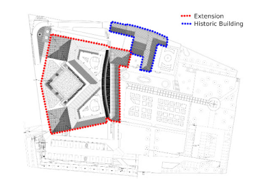
It has been obtained by the extension of a historical building. The available documentation regarding the healthcare facility and its energy systems allows dividing the building into two main areas: the historical building and the extension area. The historical building includes all the offices, while all the healthcare core activities and related services are performed within the extension area.
The extension area consists of four floors and a roof terrace. The basement is primarily for technical systems and ancillaries (electrical panel, water station, air treatment unit, etc.). The ground floor has a large area near the entrance, including reception, some offices, a bar and a small commercial area. Two hallways lead off from the main area and act as diagnostic and ophthalmology departments. They delimit a central area, including the surgical department and the intensive care unit. These areas have specific constraints in terms of ventilation and air handling. Furthermore, many electro-medical devices require electrical energy for their operation.
The first floor has two hallways similar to the ground floor but does not have a central area. This floor includes the day hospital department and outpatient activities. The second floor is structurally similar to the first but is used as an inpatient department. The activities carried out in the extension area require accurate air handling to ensure both comfort and safety standards, requiring electricity for ventilation and hot water, chilled water and steam for air conditioning. Moreover, surgical rooms and inpatient departments need access to compressed air and medical gases, which means additional electricity demand for gases and air circulation.
The thermal energy needs of the healthcare facility are fulfilled onsite through dedicated systems. The thermal power plant includes four natural gas-powered hot water generators (4 × 700 kWth) and three steam generators (3 × 202 kWth), which fulfil all the thermal energy needed for domestic hot water production and air handling systems operations. The water cooling is carried out by three water-cooled refrigeration units, which present a nominal electric power of 320 kW, with a nominal COP of 3.92. Each unit is served by two evaporative cooling towers, reaching an overall cooling capacity of 4560 kW (6 × 760 kW). The HVAC system is composed of Twentynine air handling units. It exploits hot and chilled water, steam, and electricity to carry out the air handling to ensure indoor climate conditions standards of the building.
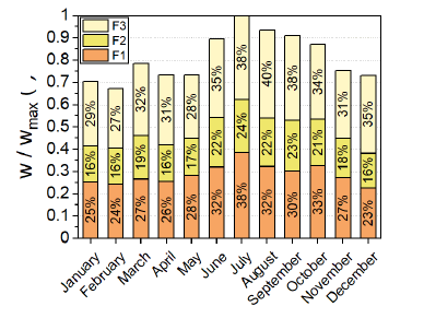
The presented study will focus on the electricity demand of the analysed healthcare facility. Analyzing the available energy provider bills allows obtaining the monthly electrical energy consumption data related to the year 2019. The electricity consumption data are generally divided by the energy provider into three timeslots, defined as:
F1, which goes from Monday to Friday, from 08:00 a.m. until 07:00 p.m. (excluding national festivity days);
F2 goes from Monday until Friday, from 07:00 a.m. to 08:00 a.m. and 07:00 a.m. to 11:00 p.m. Furthermore, F2 includes Saturday from 07:00 a.m. until 11:00 p.m.
F3 goes from Monday to Saturday, from 12:00 a.m. until 07:00 a.m. and from 11:00 p.m. until 12:00 a.m. Moreover, Sundays and national festivity are included.
[Figure 2] shows the obtained data about electricity consumption. The electricity demand presents a marked increase during the summer period. Indeed, July results to be the most energy-intensive month, presenting a +50% of February energy consumption. This significant growth can be attributed to the massive air handling requirements that characterise the summer period. This preliminary energy demand analysis shows that the electricity demand is markedly driven by the outdoor climate conditions, particularly the external temperature.
Monthly electrical energy consumption [36]
Nonetheless, the analysed data are not sufficiently detailed to obtain reliable information about the test-case energy drivers. Consequently, detailed electric energy demand data have been analysed. The energy provider specified data on the overall building electricity consumption from February 2019 until January 2020 (15-minute time step). [Figure 3] depicts the obtained data as average power curves. While there are marked differences between winter, autumn and summer electricity consumption, spring tends to be more similar to winter. [Figure 3] focuses on the daily energy demand behaviour and shows that workdays present similar characteristics regardless of the season. Starting from midnight, the electric power demand tends to remain unchanged until 6:00 a.m. Nevertheless, summer presents a nearly linear electricity demand decrease due to a gradual decrease in the air handling system exploitation corresponding to the external temperature decrease. From 06:00 a.m. to 08:30 a.m., the electricity demand progressively increases. All seasons present similar behaviours because of the increase in healthcare activity intensity.
Average power load curve behaviour during the four seasons for workdays (a), Saturday (b) and Sunday (c) [36]
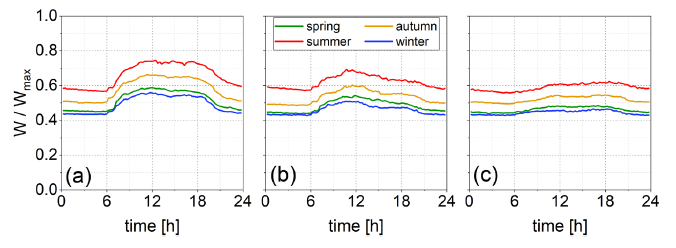
The energy demand is significantly higher when the core activities within the facility are more intense (working days from 08:30 to 18:00). All the offices and the departments are operative, leading to high electricity demand for HVAC systems, lighting, and medical equipment operations.
Morning (from 10:30 a.m. to 1:00 p.m.) and afternoon (from 4:00 to 6:00 p.m.) present higher power demand. Then, there is a mild and progressive decrease in energy demand, reaching typical night-time levels at the end of the day. On the other hand, Sundays are characterised by smoother power curves. The night behaviour of the electrical power demand tends to maintain the same behaviour found on workdays. Contrarily, the daytime does not have the marked increase typical of workdays. Moreover, the day/night transition is longer than the one found on workdays, given that the healthcare activities are less intense. Saturdays present intermediate characteristics between workdays and Sundays.
During the daytime the electricity consumption increases. Nevertheless, it reaches lower values than the ones found during the workdays. It presents a gradual decrease starting from 3:00 p.m., corresponding to the decrease in healthcare activity intensity.
The energy demand behaviour will be compared with several parameters to find the main energy drivers of the building (see [Table 1]). The considered parameters can be divided into three main categories. The time parameters are chosen to consider different time scales, such as the day's hour and the year's month. The hour of the day has been expressed through ordinal encoding, ranging between 0 and 23.75, with a 0.25 step representing 15 minutes. To maximise the correlation between the hour of the day (h) and the electrical power consumption, the former has been represented through a sine function of the h parameter. This representation allows assigning similar values to near-midnight hours that are reasonably characterised by similar electric energy consumptions. Moreover, the sine function has been shifted along the time coordinate to synchronise the sine peaks with those found in the electrical energy demand behaviour. The resulting equation is:
(7)
It is shown in eq. (8) that a similar procedure has been applied to the M (month of the year) parameter:
(8)
Description of the available features
| Feature | Description | Unit | Time step |
| Te | Outdoor air Temperature | K | 15 min |
| RH | Outdoor air Relative Humidity | % | 15 min |
| GSR | Global Solar Radiation | W/m2 | 15 min |
| p | ambient Pressure | bar | 15 min |
| WS | Wind Speed | m/s | 15 min |
| WD | Wind Direction | deg | 15 min |
| Staff srv | Staff in-Service: number of employees present in the facility during a specific day | - | 1 day |
| Hour | Hour of the day, ranging from 0 to 23.75 | 15 min | |
| Day Typ | Day Typology:1: Workday, 2: Saturday, 3: Sunday and Festivities | - | - |
| Timeslot | 1: F1, 2: F2, 3: F3 | - | - |
| Month | Month of the year, ranging from 1 to 12 | - | 1 month |
Moreover, the considered parameters include Day Typology, which separates the workdays (1) from the Saturday (2) and Sunday/Festivity (3), and Timeslot (defined in the energy provider bills), which lets to divide each week into three slots. The latter allows for treating separately the intense activity periods (e.g. daytime of the workdays) from the lesser intense activity period (night time and weekends). Information about the presence of non-medical staff was obtained from the data available in the facility. Since no data about the instantaneous values assumed by this parameter were available, the Staff in-Service (Staff srv) has been represented through a daily value. Other data like medical staff on duty or hospitalised patients were not available. The Climate Parameters includes information about the weather conditions of the same period of the electric power data, with the 15-minute time-step, and it has been made available by Consorzio LaMMA (Laboratory for Meteorology and Environmental Modelling).
Statistics of the available features
| Feature | Unit | min | MAX | mean | std dev |
| Te | K | 270.85 | 313.25 | 289.68 | 7.98 |
| RH | % | 9.00 | 100.00 | 63.06 | 22.78 |
| GSR | W/m2 | 0.00 | 1127.20 | 170.07 | 256.89 |
| p | bar | 1.0100 | 0.9780 | 1.0380 | 0.0076 |
| WS | m/s | 0.10 | 11.30 | 1.75 | 1.36 |
| WD | deg | 2.00 | 360.00 | 202.82 | 94.35 |
| Staff srv | - | 0.00 | 99.00 | 60.33 | 30.65 |
| Hour | - | 0.00 | 23.75 | - | - |
| Day Typ | - | 1 | 3 | - | - |
| Timeslot | - | 1 | 3 | - | - |
| Month | - | 1 | 12 | - | - |
[Table 2] shows statistical information about the main features taken into consideration. In particular, the following parameters have been analysed:
Te and RH are the external air temperature and the relative humidity, respectively;
GSR is the Global Solar Radiation;
p is the atmospheric pressure;
WS and WD are the Wind Speed and the Wind Direction, respectively;
Prcp represents the Precipitation in millimetres during a specific time step.
Once the data related to electrical power and energy drivers are available, it is necessary to analyse it to quantify every parameter's influence on electrical energy consumption. Correlation and regression analysis are fundamental statistical tools for this purpose. In particular, the correlation analysis lets to assess the correlation between each pair of parameters. Consequently, a correlation study has been performed on the available data related to 2019 to establish which parameters mainly influence the building energy demand behaviour.
In [Figure 4] and [Figure 5], the Pearson (r) and Spearman (ρ) correlation coefficients found between each pair of features are resumed. The table cells have been highlighted with different colours based on the value assumed by the correlation coefficients.
Pearson's product-moment correlation coefficients for the training DataSet
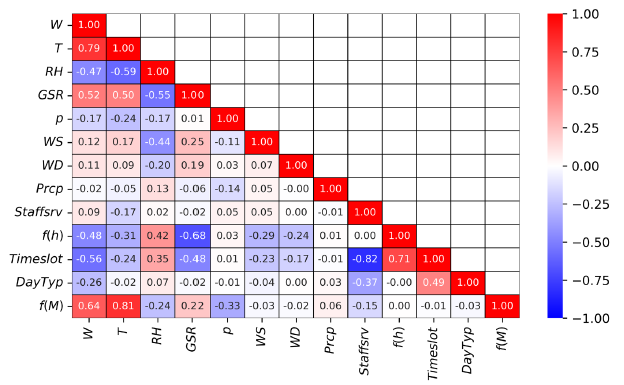
First of all, it is important to notice that the table diagonal collects the correlation coefficient of each parameter with itself, which results in a total positive linear correlation (r = 1.00, ρ = 1.00) but is not useful for identifying the main building energy drivers. Month parameter (f(M)) presents low correlation coefficients with the other time-related parameters (f(h), Day Typ and Timeslot). Contrarily, it is highly correlated with external temperature (r = 0.81, ρ = 0.82) because the monthly time scale is closer to seasons than to the daily one. Coherently, other climate parameters (Relative Humidity, Global Solar Radiation and pressure) present an intermediate correlation with the Month.
Spearman correlation coefficients for the training DataSet

Focusing on the daily time scale, the hour of the day (f(h)) presents a high correlation with the Timeslot (r = 0.71, ρ = 0.69) due to the time slot definition. As expected, it presents a high correlation also with the global solar radiation (r = −0.68, ρ = −0.79) and intermediate correlations with external temperature (r = −0.31, ρ = −0.29) and relative humidity (r = 0.42, ρ = 0.42). The Staff in-Service results highly correlated only with Timeslot (r = −0.82, ρ = −0.74) and presented an intermediate correlation with Day Typology (r = −0.37, ρ = −0.33). It can be explained considering that Staff in-Service data have a daily time step and cannot appreciate the daily time-scale variations.
More detailed data about the Staff in-Service (e.g., with a 15-minute time step) could lead to higher correlations with other time parameters, especially with the hour of the day. Further, the Staff in-Service present an intermediate correlation with external temperature (r = −0.17, ρ = −0.27) and with f(M) (r = −0.15, ρ = 0.26).
This behaviour is mainly due to the decrease of the healthcare core activities intensity during August, and it does not have statistical significance. Climate parameters, external temperature, relative humidity, and global solar radiation present relatively strong relationships between each other. Moreover, these three parameters are influenced by daily and seasonal time scales. Contrarily, other climate parameters like pressure, wind speed, wind direction and precipitations are not strictly correlated with any other considered parameter.
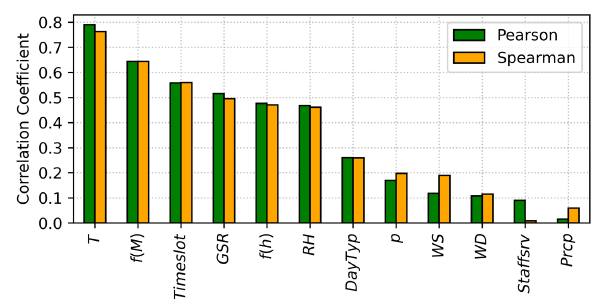
The first column in [Figure 4] and [Figure 5] presents the correlation coefficients of all the described parameters with the healthcare facility's electric power demand (W). The coefficients are also compared using a bar representation in [Figure 6]. These values are useful to identify the Energy Drivers of the healthcare facility finally. Low correlation coefficients can be found for some climate parameters (p, WS, WD, Prcp) and the Staff in-Service (Staff srv). Representing the Staff in-Service as a daily value can make it difficult to appreciate the correlation between the latter and the electrical power demand. The results show a weak correlation (r = 0.09) with the target (W), confirming that the staff occupancy does not significantly affect the electrical power demand.
As described in the section METHODS, the filter method is realised to identify irrelevant and redundant features. Irrelevant features are characterised by a weak correlation with the target, while a feature can be considered redundant when it presents a high correlation coefficient with another input feature.
Pearson and Spearman correlation coefficients between building electricity demand and the available input features
Consequently, it is fundamental to choose the thresholds for use in identifying these two feature typologies. In literature [39], some examples of threshold choices are provided. Nevertheless, the thresholds mentioned above are only literature-suggested values. One should chose the thresholds for a specific application as a compromise between prediction accuracy and computational efficiency.
The irrelevant features can be found by defining a threshold for the correlation coefficients between the input features and the electricity demand of the healthcare facility. All the input features that present coefficients higher than the chosen threshold will be included in the following steps of the work. The threshold has been carefully chosen to avoid the accidental elimination of useful features but to reduce the number of features considered for the following analyses. Consequently, all the features that present both Pearson and Spearman correlation coefficients lower than 0.1 are considered "Irrelevant Features" and will be excluded from the input dataset. The Staff in-Service (Staff srv) and Precipitation (Prcp) features result are irrelevant features based on the described procedure. This fact can be corroborated by considering that the main part of the electricity consumption of the healthcare facility is due to the HVAC systems.
Air handling is mainly used for internal climate control of healthcare core activity areas. It aims to maintain security standards imposed by the Italian regulations and ensure continuous temperature and humidity control in the diagnostic department, which houses constantly operating electro-medical equipment. Consequently, the people's occupancy contributes a negligible ion to the increase in energy consumption.
Once the irrelevant features have been identified, a second check must be made to exclude redundant features. In the literature [39], an upper bound of 0.9 is chosen as a threshold for the correlation coefficient between each pair of input features. The analysed dataset does not present any redundancy based on this coefficient.
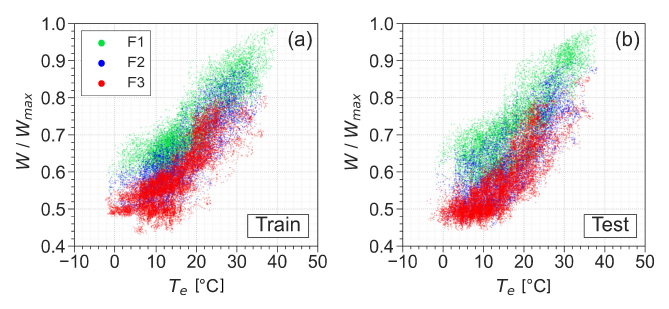
The remaining features are then used to perform a further step of feature selection by directly applying the multiple linear regression (MLR). Moreover, [Figure 7] shows that the electrical power demand of the healthcare facility appears to be in a quadratic relationship with the external temperature. The squared temperature () has been included as an input feature of the MLR model to include that quadratic relationship in the present analysis.
Electrical Power Demand of the Healthcare Facility vs External Temperature from 02/06/2019 until 02/05/2020 (a) and from 02/06/2020 until 02/05/2021 (b)
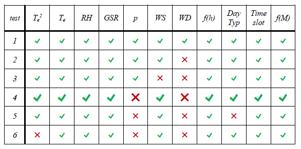
The method has been applied to the already described dataset by conducting several tests. The aim was to minimise the number of input features and avoid reducing the model's prediction performance. First, the Multiple Linear Regression model has been trained using all features accepted by the previous filter method to obtain a reference model. Then, further tests were carried out. Several pieces of training have been performed, removing consecutively all the features that had an intermediate or low correlation with the electrical power demand (see [Table 3]). The feature removing procedure was carried out by proceeding from the feature with the lowest correlation coefficient to the one with the highest. If removing a feature causes an increase of the MSE greater than 0.5% of its reference value, the feature will be re-integrated into the next test. To quantify the MSE variation, the parameter ΔMSE has been calculated as follows:
(9)
where MSE is the Mean Squared Error defined in eq. (4) and i represents the current test (see [Table 3]). Practically, ΔMSE represents the variation of the mean squared error (expressed in percentage) of the current test in comparison to the one found in the preceding step.
As already said, the first test (Test 1 in [Table 3] and [Figure 8]) has been carried out by considering all the accepted features described in the preceding section (excluding Staff srv and Prcp). It presents a good performance in electric energy forecasting, resulting in an adjusted R2 of 0.836. The obtained model will serve as a reference for the following tests. Since the Wind Direction (WD) results as the feature with the lowest correlation coefficient with the absorbed power, it has been removed to perform the second test. As expected, the MSE saw an increase of only 0.044%.
Evaluation parameters for the MLR tests carried out in the study
| Test | Adjusted R2 | ΔMSE% | Removed Variable |
| 1 | 0.83633 | - | - |
| 2 | 0.83636 | 0.044% | WD |
| 3 | 0.83449 | 0.911% | WS |
| 4 | 0.83631 | 0.035% | p |
| 5 | 0.83505 | 0.763% | Day Typ |
| 6 | 0.83349 | 1.233% |
As shown in [Table 3], the following tests highlight that removing WS, Day Typ and causes a non-negligible increase in MSE. On the other hand, the WD and p features do not improve the prediction performance of the regression model and have been removed from the final dataset. At the end of the presented procedure, the chosen model is composed of nine features of the available thirteen and can be represented as:
(10)
Selected variables for each test carried out
Coefficients of the selected Multiple Linear Regression Model
| Coefficient | Value | Coefficient | Value |
| c0 | 15.434011 | cWS | −0.033398 |
| 19.386580 | ch | −0.015338 | |
| −33.892952 | cdt | −0.030019 | |
| cRH | 0.027181 | cts | −0.123984 |
| cGSR | −0.013621 | cM | 0.034358 |
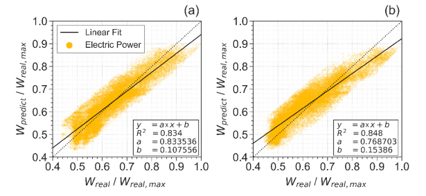
[Table 5] resumes the coefficients seen in eq. (10). The model prediction performance is similar to the reference one (Test 1), showing an increase in MSE of approximately 0.035%. The parameters selection allowed one to choose the useful features to improve the prediction capabilities of the MLR model. The selected model has been then applied to a test dataset related to the period between 02/06/2020 and 02/05/2021 constituted by the same features analysed for the training set. [Figure 9] compares the instantaneous real electrical power demand of the healthcare and the one predicted by the MLR model for both the training and test period. A model which perfectly predicts the electrical power demand should generate a series of points coinciding with the diagonal of the graphics (black dotted lines).
The applied model tends to have a uniform variation around the diagonal, particularly regarding the training period. Furthermore, [Figure 9] reports the linear fit of the represented data. The linear fit shown in [Figure 9a] illustrates an R2 equal to 0.834 around the dotted line, representing an intercept of 0.108 and a slope of 0.834. The two lines intersect at W/Wreal, max equal to 0.646, meaning that the model tends to overestimate the power consumption below this value. For higher values, the predicted electrical power demand results lower than the real one. [Figure 9b] represents the model application on the test dataset. One can notice that the critical W/Wreal, max is higher than the one found in the training dataset and equals 0.665. Moreover, the behaviour found previously is similar, but more pronounced. One could predict that situation, considering the model has been realised through the training set (see [Figure 9a]) and consequently a better prediction quality on those data is expected.
Multiple Linear Regression model results applied to the training dataset (a) and the test dataset (b)
The energy characterisation of a system can be difficult if it is prone to changes in energy usage over time. Indeed, energy consumption can change over time, maintaining the same energy drivers' behaviour. This can be due to changes in the building activity or systems management strategy. If, on the one hand, an increase in energy consumption due to a malfunction of the systems may be evident, other kinds of changes in energy consumption can be mild and difficult to find through an analysis of the simple historical data of building energy consumption. Consequently, it is pivotal to apply methods enabling better to highlight little and progressive increase in energy consumption behaviour. The proposed method's final step consists of exploiting the obtained MLR model to realise a CUSUM control chart (see section METHODS).
The CUSUM chart shown in [Figure 10] has been divided into two parts. The first (blue line) represents the training period, whose data were used to realise the MLR model. The S standard deviation (σs), calculated for that period has been used to establish the range in which S variation will be considered regular (±3×σs). In other words, the training period has been taken as a reference for the S variability. As expected, the S value of the reference period fluctuates around the null value, returning to zero at the end of the reference period.
The test period starts on 02/06/2020. As seen from the red line in [Figure 10], the S value starts an almost constant decrease from this time step until the end of June 2020. This fact means that the electrical power demand of this period is generally lower than the standard one, resulting in lower consumption of the healthcare facility compared to the standard one. The healthcare core activities were mildly affected by the COVID-19 emergency, resulting in a slight reduction in the outpatient activities and a more pronounced reduction in the restoration activities. This activity trend reduces the energy demand directly related to the mentioned areas, also causing a reduction in the exploitation of the corresponding Air Handling Units.
Furthermore, at the beginning of February 2020, the progressive substitution has been started of all the filtering systems related to the Air Handling Units. The substitution continued until the third week of March 2020, causing a reduction in the electrical power demand of the Air Handling System. Despite the mild change in energy exploitation and management during this period, the presented method can highlight it through the continuous decrease of the red line in [Figure 10]. In the period between July 2020 and September 2020, an increase in electricity consumption compared to the reference period occurs, resulting in a continuous increase of S. First, at the beginning of July 2020, the Building Energy Management System (BEMS) encountered technical problems which entailed malfunctions in the Air Handling System management strategy, causing an increase in the electrical energy consumption of the Air Handling Unit fans and, consequently, of all the related systems (refrigerators, Cooling Towers). Moreover, the refrigerators have experienced malfunctions which led to a reduction in their electrical efficiency.
Cumulative Sum of Differences for training (blue line) and testing periods (red line)
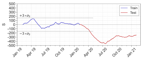
In September 2020 an optimisation campaign has been carried out on the Air Handling System, which brought back its normal functioning. In addition, maintenance operations on the refrigerators restored their standard efficiency. A new restoration area served by two new Air Handling Units was activated in September 2020. Looking at [Figure 10], from the beginning of October 2020 until the end of the test period, electricity demand maintains the same behaviour.
One can conclude that the optimisation campaign was successful, achieving a reduction in the Air Handling System electricity consumption and compensating for the physiological increase in consumption due to the introduction of the systems above.
The study has been carried out by analysing electrical energy consumption data from February 2019 until January 2020, taken as standard building energy demand. Several climate and activity parameters have been included in the analysis by carrying out a correlation analysis, which allows the authors to quantify the influence that each analysed parameter has on the electrical energy consumption of the Healthcare Facility. Consequently, it is possible to select the main building energy drivers.
The knowledge obtained from the correlation study has been exploited to develop a Multiple Linear Regression model. In particular, a function has been obtained for predicting the building electric energy consumption based on the values assumed by the selected parameters during a specific time step. Since the model has been trained using data related only to the standard period, it can be exploited to calculate the healthcare standard electricity demand. As a result, the study led to the development of an offline monitoring method applicable to the future healthcare energy requirements to find any change in the electricity consumption trend of the healthcare facility. The comparison of actual electricity consumption with standard one led to the creation of a CUSUM control chart.
The proposed method allows to find any variation of the actual electric energy consumption compared to the standard one. It could be a useful tool to monitor the energy efficiency of a building and its plants and systems. Furthermore, the numerical method makes it applicable to different test cases and scenarios. For example, the model can be applied to more specific electrical power demand data for obtaining more detailed information about the energy consumption behaviour of specific building areas or sub-systems. Possible future improvements in the energy system's control strategy can be identified, aiming at a continuous optimisation of the building energy requirements.
| e | residual | |
| h | hour of the day | |
| M | month of the year | |
| r | Pearson's correlation coefficient | |
| R2 | coefficient of determination | |
| S | cumulated sum | |
| T | temperature | [°C] or [K] |
| w | electrical energy | [kWh] |
| W | electrical power | [kW] |
| Greek letters | ||
| σ | standard deviation | |
| ρ | Spearman's correlation coefficient | |
| Subscripts and superscripts | ||
| Adj | Adjusted | |
| E | External, Outdoor | |
| Max | Maximum | |
| Abbreviations | ||
| AE | Absolute Error | |
| BEM | Building Energy Modelling | |
| BEMS | Building Energy Management System | |
| HVAC | Heating, Ventilation and Air Conditioning | |
| MAE | Mean Absolute Error | |
| MLR | Multiple Linear Regression | |
| MSE | Mean Squared Error | |
- ,
Analysis of Building Energy Consumption in a Hospital in the Hot Summer and Cold Winter Area ,Energy Procedia , Vol. 158 ,pp 3735–3740 , 2019, https://doi.org/https://doi.org/10.1016/j.egypro.2019.01.883 - ,
Electrical and thermal energy in private hospitals: Consumption indicators focused on healthcare activity ,Sustainable Cities and Society , Vol. 47 ,pp 101482 , 2019, https://doi.org/https://doi.org/10.1016/j.scs.2019.101482 - ,
Indoor hospital air and the impact of ventilation on bioaerosols: a systematic review ,Journal of Hospital Infection , Vol. 103 (2),pp 175–184 , 2019, https://doi.org/https://doi.org/10.1016/j.jhin.2019.06.016 - ,
Thermal environment in Swedish hospitals: Summer and winter measurements ,Energy and Buildings , Vol. 37 (8),pp 872–877 , 2005, https://doi.org/https://doi.org/10.1016/j.enbuild.2004.11.003 - ,
Energy Efficiency Index of Ambulatories and Hospitals ,International Journal of Control Theory and Applications , Vol. 9 ,pp 59–64 , 2016 - ,
Energy Cost and Consumption in a Large Acute Hospital ,International Journal On Architectural Science , Vol. 5 , 2004 - ,
‘Study of different cogeneration alternatives for a Spanish hospital center’ ,Energy and Buildings , Vol. 38 (5),pp 484–490 , 2006, https://doi.org/https://doi.org/10.1016/j.enbuild.2005.08.011 - ,
Assessing the energy consumption for heating and cooling in hospitals ,Energy and Buildings , Vol. 48 ,pp 146–154 , 2012, https://doi.org/https://doi.org/10.1016/j.enbuild.2012.01.022 - ,
‘A quantitative analysis of final energy consumption in hospitals in Spain’ ,Sustainable Cities and Society , Vol. 36 ,pp 169–175 , 2018, https://doi.org/https://doi.org/10.1016/j.scs.2017.10.029 - ,
Impact of climate change on demands for heating and cooling energy in hospitals: An in-depth case study of six islands located in the Indian Ocean region ,Sustainable Cities and Society , Vol. 44 ,pp 629–645 , 2019, https://doi.org/https://doi.org/10.1016/j.scs.2018.10.031 - ,
Thermal comfort standards, measured internal temperatures and thermal resilience to climate change of free-running buildings: A case-study of hospital wards ,Building and Environment , Vol. 55 ,pp 57–72 , 2012, https://doi.org/https://doi.org/10.1016/j.buildenv.2011.12.006 - ,
Resilience of "Nightingale" hospital wards in a changing climate: ,Building Services Engineering Research and Technology , 2012, https://doi.org/https://doi.org/10.1177/0143624411432012 - ,
Equipment and Energy Usage in a Large Teaching Hospital in Norway ,Journal of Healthcare Engineering , 2015https://www.hindawi.com/journals/jhe/2015/231507 - ,
Electricity consumption of medical plug loads in hospital laboratories: Identification, evaluation, prediction and verification ,Energy and Buildings , Vol. 107 ,pp 392–406 , 2015, https://doi.org/https://doi.org/10.1016/j.enbuild.2015.08.022 - ,
Environmental Impacts of the U.S. Health Care System and Effects on Public Health ,PLOS ONE , Vol. 11 (6),pp e0157014 , 2016, https://doi.org/https://doi.org/10.1371/journal.pone.0157014 - ,
Heat pipe heat exchanger for heat recovery in air conditioning ,Applied Thermal Engineering , Vol. 27 (4),pp 795–801 , 2007, https://doi.org/https://doi.org/10.1016/j.applthermaleng.2006.10.020 - ,
Toward cost-effective and energy-efficient heat recovery systems in buildings: Thermal performance monitoring ,Energy , Vol. 137 ,pp 487–494 , 2017, https://doi.org/https://doi.org/10.1016/j.energy.2017.02.159 - ,
Experimental analysis of an air-to-air heat recovery unit for balanced ventilation systems in residential buildings ,Energy Conversion and Management , Vol. 52 (1),pp 635–640 , 2011, https://doi.org/https://doi.org/10.1016/j.enconman.2010.07.040 - ,
Energy savings by energy management systems: A review ,Renewable and Sustainable Energy Reviews , Vol. 56 ,pp 760–777 , 2016, https://doi.org/https://doi.org/10.1016/j.rser.2015.11.067 - ,
Bi-level energy-efficient occupancy profile optimisation integrated with demand-driven control strategy: University building energy saving ,Sustainable Cities and Society , Vol. 48 ,pp 101539 , 2019, https://doi.org/https://doi.org/10.1016/j.scs.2019.101539 - ,
Low impact energy saving strategies for individual heating systems in a modern residential building: A case study in Rome ,Journal of Cleaner Production , Vol. 214 ,pp 791–802 , 2019, https://doi.org/https://doi.org/10.1016/j.jclepro.2018.12.320 - ,
Heating and cooling energy trends and drivers in buildings ,Renewable and Sustainable Energy Reviews , Vol. 41 ,pp 85–98 , 2015, https://doi.org/https://doi.org/10.1016/j.rser.2014.08.039 - ,
Building energy efficiency for public hospitals and healthcare facilities in China: Barriers and drivers ,Energy , Vol. 103 ,pp 588–597 , 2016, https://doi.org/https://doi.org/10.1016/j.energy.2016.03.039 - ,
An insight into actual energy use and its drivers in high-performance buildings ,Applied Energy , Vol. 131 ,pp 394–410 , 2014, https://doi.org/https://doi.org/10.1016/j.apenergy.2014.06.032 - ,
A review on modeling and simulation of building energy systems ,Renewable and Sustainable Energy Reviews , Vol. 56 ,pp 1272–1292 , 2016, https://doi.org/https://doi.org/10.1016/j.rser.2015.12.040 - ,
Modeling and Simulation of Energy Systems: A Review ,Processes , Vol. 6 (12), 2018, https://doi.org/https://doi.org/10.3390/pr6120238 - ,
Energy models for demand forecasting—A review ,Renewable and Sustainable Energy Reviews , Vol. 16 (2),pp 1223–1240 , 2012, https://doi.org/https://doi.org/10.1016/j.rser.2011.08.014 - ,
Comparison of neural network, conditional demand analysis, and engineering approaches for modeling end-use energy consumption in the residential sector ,Applied Energy , Vol. 85 (4),pp 271–296 , 2008, https://doi.org/https://doi.org/10.1016/j.apenergy.2006.09.012 - ,
Modeling of end-use energy consumption in the residential sector: A review of modeling techniques ,Renewable and Sustainable Energy Reviews , Vol. 13 (8),pp 1819–1835 , 2009, https://doi.org/https://doi.org/10.1016/j.rser.2008.09.033 - ,
Using regression analysis to predict the future energy consumption of a supermarket in the UK ,Applied Energy , Vol. 130 ,pp 305–313 , 2014, https://doi.org/https://doi.org/10.1016/j.apenergy.2014.05.062 - ,
Application of Statistical and Artificial Intelligence Techniques for Medium-Term Electrical Energy Forecasting: A Case Study for a Regional Hospital ,Journal of Sustainable Development of Energy, Water and Environment Systems , Vol. 8 (3),pp 520–536 , 2020, https://doi.org/https://doi.org/10.13044/j.sdewes.d7.0306 - ,
Prediction and optimisation of energy consumption in an office building using artificial neural network and a genetic algorithm ,Sustainable Cities and Society , Vol. 61 ,pp 102325 , 2020, https://doi.org/https://doi.org/10.1016/j.scs.2020.102325 - ,
Building Behavior Simulation by Means of Artificial Neural Network in Summer Conditions ,Sustainability , Vol. 6 (8), 2014, https://doi.org/https://doi.org/10.3390/su6085339 - ,
Using EnergyPlus to Simulate the Dynamic Response of a Residential Building to Advanced Cooling Strategies ,pp 10 , - ,
Residential Sector Energy Demand Estimation for a Single-family Dwelling: Dynamic Simulation and Energy Analysis ,Journal of Sustainable Development of Energy, Water and Environment Systems , Vol. 9 (2),pp 1-18 , 2021, https://doi.org/https://doi.org/10.13044/j.sdewes.d8.0358 - ,
CUSUM quality control chart for monitoring energy use performance , 2007, https://doi.org/https://doi.org/10.1109/IEEM.2007.4419388 - ,
Energy performance measurement, monitoring and control for buildings of public organisations: Standardised practises compliant with the ISO 50001 and ISO 50006 ,Developments in the Built Environment , Vol. 4 ,pp 100024 , 2020, https://doi.org/https://doi.org/10.1016/j.dibe.2020.100024 - ,
Reconstruction and Analysis of the Energy Demand of a Healthcare Facility in Italy ,E3S Web Conf , Vol. 197 ,pp 02009 , 2020, https://doi.org/https://doi.org/10.1051/e3sconf/202019702009 - ,
A systematic feature selection procedure for short-term data-driven building energy forecasting model development ,Energy and Buildings , Vol. 183 ,pp 428–442 , 2019, https://doi.org/https://doi.org/10.1016/j.enbuild.2018.11.010 - ,
Linear regression models, least-squares problems, normal equations, and stopping criteria for the conjugate gradient method ,Computer Physics Communications , Vol. 183 (11),pp 2322–2336 , 2012, https://doi.org/https://doi.org/10.1016/j.cpc.2012.05.023 - ,
Adjusted R-squared type measure for exponential dispersion models ,Statistics & Probability Letters , Vol. 80 (17),pp 1365–1368 , 2010, https://doi.org/https://doi.org/10.1016/j.spl.2010.04.019