


Small-scale biomass-based cogeneration has the potential to contribute significantly to solving the challenges Europe faces while pursuing to make its energy system smart, clean, flexible, secure, efficient and cost competitive. High efficiencies are achieved by combining heat and power generation; even cooling can be integrated into the such concept. Small-scale cogeneration is considered a technology that provides flexibility to future energy systems by balancing variable intermittent renewable energy sources. Such plants may be designed and implemented in mobile applications.
Biomass-based cogeneration has received increasing attention in energy development policy [1]. Bio-oil-based combined heat and power (CHP) is, after heat-only application, the second most economically competitive application in six European countries [2]. Researchers addressed optimal sizing, optimisation [3], and energy and exergy efficiencies of such plants [4]. Effective integration of such cogeneration in future energy systems requires a high level of overall energy efficiency and low flue gas emissions over the whole range of operating conditions [4]. A smart, demand-driven unit should be capable of dealing with the fluctuating energy demand and/or varying availability of wind/solar power [5]. Moreover, a highly flexible ratio between heat and power generation is always desired to achieve high resource efficiencies. Dynamic modelling and predictive simulation are useful in designing, controlling, and optimising technology-intensive engineering systems. For example, in [6], a simulation model shows how a solar heating system can be efficient for building heating. With the aid of a dynamic plant model, the performance of a wastewater treatment plant after upgrading with tertiary treatment is predicted, and its design is improved [7].
The general goal of this study is an optimisation and smart control of a cogeneration plant fuelled with fast-pyrolysis bio-oil (FPBO). The primary objective of this study is to develop, parameterise and tune a dynamic model of the cogeneration plant. The secondary objective is to simulate and analyse plant performance and energy efficiency and characterise heat/power generation coupling. The system is a hybrid diesel generator/flue gas boiler plant for electricity generation and water/space heating. The plant has two unique features: (i) FPBO is the new fuel for both engine and boiler and influences their operation and emissions, (ii) the oxygen content of engine flue gas is the only oxidiser for FPBO combustion in the boiler's burner, and consequently, power and heat generation are partially decoupled or nonlinearly correlated. These features affect the operation and, in turn, the dynamic response of the plant. Therefore, the research objective is to modify, customise, and re-parameterise the existing dynamic models of the components from the previously published literature, and validate them with new measurements from cogeneration components running on FPBO. The focus is on developing a control-oriented dynamic model of the cogeneration plant. The study presents the integration of the components' dynamic models into a predictive system model. The input-output relations of different components and their interfaces are modelled and included in the system model. Simple preliminary controls are designed and included in the system model to make model simulations conform with available measurements, and their performances are evaluated.
The rest of this paper is organised as follows. The next section presents the motivation, a literature review of the study subject and the contributions of this paper, followed by a brief description of the cogeneration plant under study. Then, an overall view of the system model, its components and what is modelled is depicted. Main sub-models are also presented, including control-oriented models of diesel engine, flue gas boiler, and SCR unit. The design of preliminary controls and parameter tuning is presented next. Predictive simulations illustrate the applicability and usefulness of the dynamic model for cogeneration system analysis. The paper ends with findings and conclusions.
The studied cogeneration plant aims at highly flexible cogeneration, implying the plant can adjust heat generation between the minimum and maximum levels at all the engine electrical loads (heat/electricity ratio between 2 and 10). A smart control unit is needed to exploit such flexibility. Developing a dynamic system model is the first step toward such a control unit. The dynamic model enables the design and evaluation of the controllers at the components and system levels. The dynamic model can evaluate various operating points at different operating modes and scenarios to find optimal working conditions. The model is also useful as a part of the plant's digital twin during its normal operation. Finally, the dynamic model is a useful tool to predict demand response, components utilisation rates, and their energy efficiencies when the plant generates energy for a certain use case of cogeneration (e.g., hospitals, commercial buildings, greenhouses, etc.). These parameters are inputs for a financial and feasibility study of such concepts before their large-scale roll-out.
Research work on modelling individual components of a cogeneration system is extensive. The automotive and energy sectors are precursors for diesel engine modelling, control, and supervision. A comprehensive collection of modelling approaches for internal combustion engines is available in [8]. As a predominant modelling approach for control design, mean-value modelling of gas exchange in diesel engines is presented by [9]. Reference [10] reviewed modelling, control and supervision systems applied in internal combustion engines. Dynamic modelling of water heating boilers has also been addressed in the literature [11]. An essential component in the boiler system is its burner, as it determines the combustion and thermodynamic properties of the flue gas. Some studies addressed the optimisation of swirl burners running on biofuels and experimentally derived models of thermal efficiency and losses [12]. Control-oriented models of the cleaning system components, including Diesel Particulate Filter [13] and Selective Catalytic Reduction [14], are also available to complement the dynamic model of a cogeneration plant. The dynamic model of SCR is used for fault-tolerant control design [15] and fault diagnostics of SCR systems [16].
The literature review focuses on hybrid cogeneration systems based on internal combustion prime movers, e.g., diesel generators or gas microturbines. Only this aspect defines the plant, and other aspects such as being a hybrid with a flue gas boiler, integrating a flue gas cleaning system, and operating on biofuel are relaxed. The search keywords are every combination of "simulation, dynamic model, and mathematical model" and "cogeneration, hybrid power system, combined heat and power".
Cogeneration of power and heat can be coupled or decoupled [17]. In a coupled system, heat generation is a by-product of electricity generation and is linearly correlated [18]. Decoupled cogeneration involves additional heat or electricity generating/storage components, e.g., boiler, heat pumps [19], solar power [20], solar thermal, wind turbine, and batteries [21]. Adding a new component sometimes imposes more challenges on the plant modelling task depending on the interaction of the new component with existing ones [22]. For instance, solar power could be a backup for a diesel generator or vice versa. Adding solar power, wind power, and batteries affects the electric part and the connection to the smart grid. Boilers and heat pumps must integrate the thermal part or flue gas path. In this regard, the SmartCHP cogeneration plant of this study is nonlinearly coupled or semi-decoupled. Therefore, the existing models for coupled or decoupled systems might not be adequate for dynamic modelling and optimisation. There is a need to develop models compatible with the unique features of this cogeneration concept.
Some micro-CHP models used for plant optimisation build on steady-state experimentally derived static maps of system components' operation [23]. Heat and electricity production dynamics are simulated using a generic grey-box model with few and easily accessible parameters [18]. Such maps represent emissions, useful outputs, efficiency, and fuel consumption as functions of engine operating characteristics [24]. For instance, in [25], the total efficiency of a Stirling engine in a given mode is defined as a function of the return water temperature, or in [26], for the prime movers of CHP, the hourly fuel consumption rate is determined using polynomial fits of engine load. Another approach for modelling diesel generators is to use first-order [27] or second-order [28] transfer functions with gains and time-delay parameters. The ability of transfer function models to incorporate the effects of fuel characteristics, flue gas flow rate and mixture is limited.
On the other hand, detailed modelling of the subcomponents of a combustion-based micro-CHP enables part-load performance characteristics and control system performance to be investigated [29]. Moreover, different possibilities for the variation of the thermal-to-power ratio can be analysed [30]. For example, a detailed combustion engine modelling includes cylinder wall heat transfer and intake/discharge gas exchange processes. Detailed dynamic models also enable incorporating the interaction of a user and its surrounding environment with a micro-CHP plant, such as user load profile [31], water and space heating temperature preference, or the surrounding air temperature [32]. Moreover, the effect of the operating mode of the prime movers, such as steady-state, warm-up and shut down, on power and thermal production and energy efficiencies may be investigated [33]. In [34], the model of an engine-based cogeneration system can predict the fuel use, thermal output, and electrical generation of a cogeneration device in response to changing load, coolant temperature and flow rate, and control strategies. This paper employs a detailed modelling approach of the hybrid cogeneration system, i.e., diesel generator/boiler/gas treatment system, to enable such investigations.
The contribution of this paper is twofold. Firstly, it starts with the dynamic models developed for similar components by already published studies. Then it modifies, parameterises, and fine-tunes the models to fit best with the modified diesel engine and the newly designed swirl flue gas burner. The models are fine-tuned with experimental data from these two components operating on FPBO. It is the new fuel for both systems and has challenging characteristics for combustion in the existing CHP components. FPBO contains about 20 % water and is viscous and acidic. Therefore, its combustion and the products from its combustion differ from those of diesel fuels. The models for the oxygen content of flue gas and NOx emissions are particularly parameterised based on the unique characteristics of FPBO. Secondly, the developed dynamic model incorporates the unique design of the cogeneration plant, which calls for new process modelling. For example, the flue gas burner uses only the oxygen of engine flue gas as its oxidiser, which affects FPBO combustion and emissions from the burner. Due to the high availability of oxygen in the flue gas at a low engine load, the boiler has more freedom to produce a wide range of thermal power. Whereas, at a high engine load, low oxygen availability limits the boiler, which cannot effectively produce heat. A semi-decoupled cogeneration concept with a nonlinear relationship between heat and power generation appears relevant. Heat losses in different plant sections are also a function of FPBO combustion. These aspects necessitate new dynamic modelling at both the components and system levels. To the best of our knowledge, there is no dynamic model published in the literature that could be used or fit directly for predictive simulation of this plant.
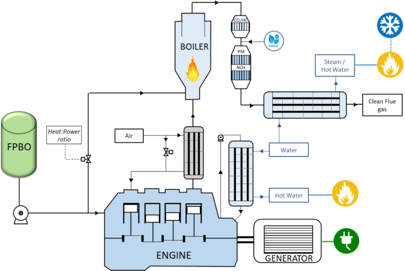
The technical concept of the cogeneration plant is presented in Figure 1. Heat and power generation are combined in a hybrid diesel generator and flue gas boiler system. One unique and new feature of this plant is that it is fuelled with fast-pyrolysis bio-oil (FPBO) originating from different types of biomasses. Fast pyrolysis converts biomass into a uniform liquid intermediate called FPBO, and high feedstock flexibility characterises the process. Nowadays, FPBO is produced on a commercial scale in Europe.
The input air is heated before entering the diesel engine through a heat exchanger that recovers heat from diesel engine flue gas. FPBO is combusted in the diesel generator to generate heat and power. Heat is extracted from the engine jacket and carried by engine coolant through a heat exchanger. The flue gas burner/boiler solely uses engine flue gas's oxygen content to combust FPBO. Depending on heat and power demand profiles, either only the CHP engine is operating, or both the engine and burner are on. When power demand is high and heat demand is low, there is no need to generate extra heat, and only the diesel generator will be operating, and the burner will be off. If heat demand is high and power load is low, heat from the CHP engine might not be enough to cover heat demand; therefore, extra heat will be generated by the burner/boiler. The hybrid diesel generator - flue gas boiler system provides a flexible heat-to-power ratio. In this sense, the plant is a flexible cogeneration unit that can deal with the fluctuating energy demand and varying wind/solar power availability.
The plant also includes a newly designed flue gas cleaning system downstream of the boiler. It includes oxidation catalyst (OC), which reduces carbon monoxide (CO) and unburned hydrocarbons (HC), diesel particulate filter (DPF), which reduces particulate matter (PM) and CO and HC, if any, and selective catalytic reduction (SCR) with urea for NOx reduction. Urea solution is injected upstream of SCR into the flue gas stream. Heat is extracted from the cleaned flue gas by heat exchangers or condensation units. In the current research project, SmartCHP [35], a prototype of such a plant is under development.
SmartCHP concept [35]
The research method, as presented in Figure 2 and Table 1, is formulated to serve the research objective. This objective is to develop, parameterise, and tune a dynamic model of the cogeneration plant. First, the inputs and output variables of the model are defined. Then the procedure to implement the system model is outlined.
Major inputs and outputs of the simulation model
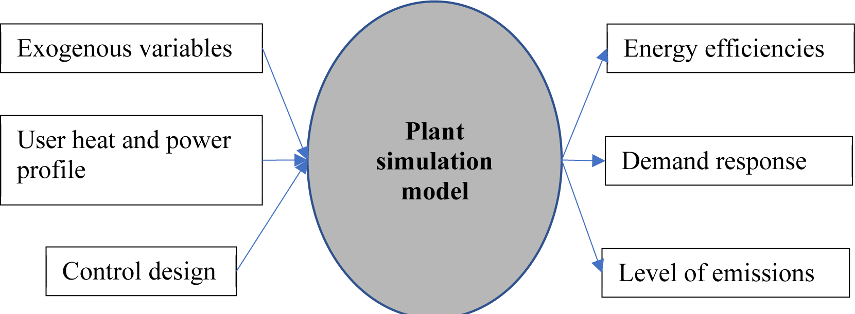
Table 1 explains the research method's elements and the procedures to implement the models. More details of research elements follow in the next sections.
Description of research elements
Element |
Sub-elements/description |
||
|---|---|---|---|
Objective |
Develop, parameterise, and tune a dynamic model of the cogeneration plant |
||
Exogenous variables |
|
||
User heat and power profile |
Hourly heat and power demands in [kW] |
||
Control design |
|
Energy efficiencies |
|
Demand response |
Fulfilled and unfulfilled demands, model outputs compared with demands |
||
Emission level |
CO, NOx, and HC emissions downstream of the cleaning system discharged from the plant |
||
Plant simulation model |
Procedure outline:
|
The cogeneration system consists of a diesel generator, a flue gas boiler, a dedicated flue gas cleaning system, and a heat exchanger and condensers. The focus here is on the flue gas path and simulating the behaviour of system components most affected by the biofuel properties and the resulting flue gas characteristics, i.e., its temperature and its composition. Figure 3 shows the system configuration that reflects this focus point and indicates the state variables of the components. The diesel generator, represented only by diesel engine components on the flue gas path, includes fresh air heating, compressor, intake receiver, cylinders, outlet receiver, and turbine. It is noted that engine rotational speed - the parameter describing engine and alternator interface - is present in the system model. An adaptive PI controller regulates the FPBO injection to keep the engine speed constant at 1500 RPM.
SmartCHP system configuration, components, and their interfaces
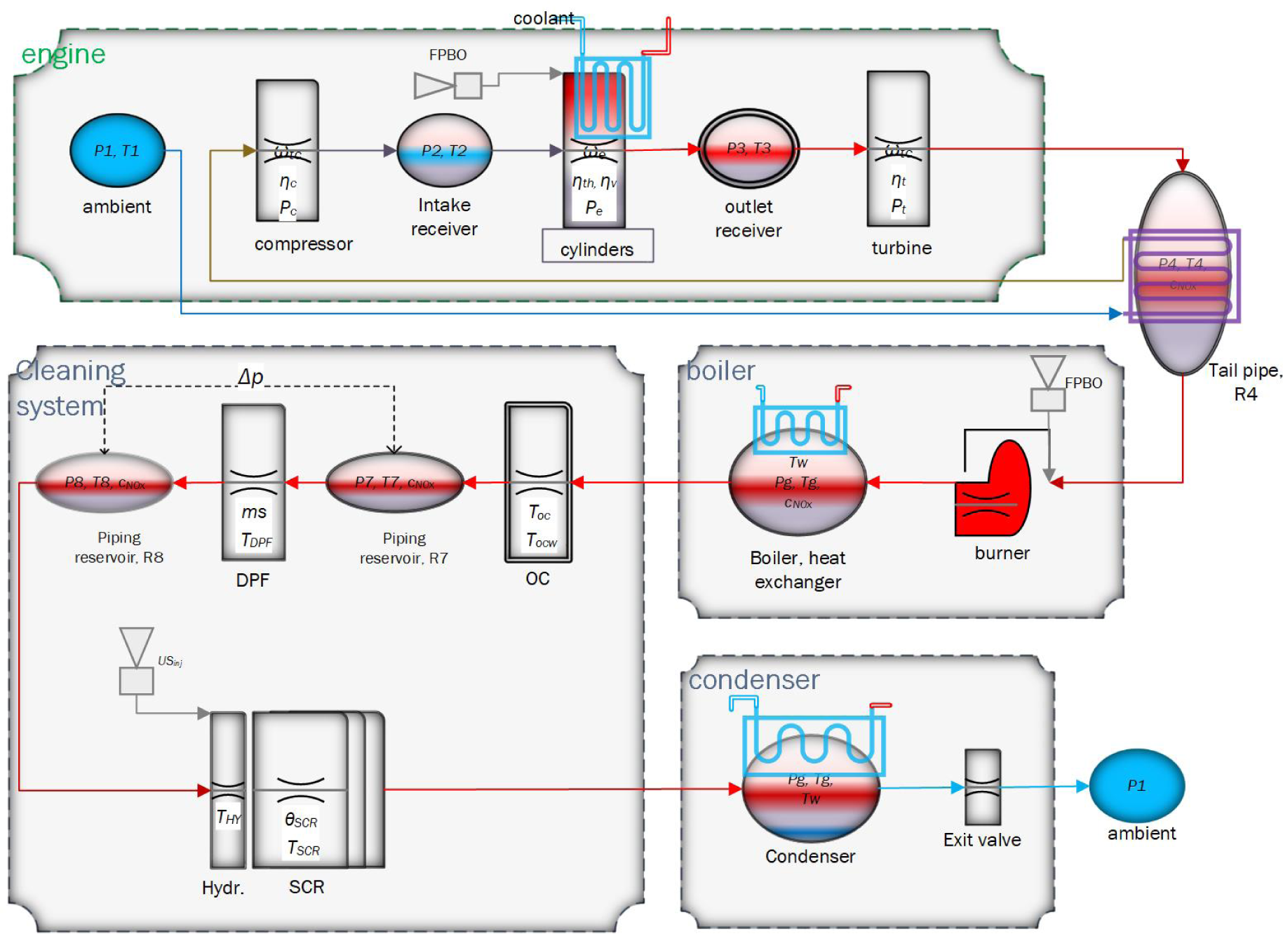
The next component is the flue gas boiler with a burner running on FPBO and using the remaining engine flue gas oxygen as an oxidiser. The interface between the burner and diesel engine is the tail pipe R4, which is modelled as a reservoir element and allows for modelling the backpressure by the burner or by the cleaning system in the case engine flue gas is directed to the cleaning system and the boiler is bypassed. The boiler model includes a hot water heat exchanger.
The flue gas from the boiler finds its way to the cleaning system. The first component is OC, which may affect the NO2/NOx ratio. After OC, the DPF is placed that might cause significant backpressure due to the accumulation of PM inside it. This backpressure is modelled by the reservoir component R7 placed between OC and DPF. The last component in the cleaning system is the SCR unit. It consists of a hydrolysis part where the injected urea solution vaporises and forms a flow of NH3 and SCR cells where NOx is reduced by the NH3 absorbed on the surface of the SCR catalyst. Last, a condensation unit downstream of the cleaning system absorbs heat from flue gas. The system model also includes the dynamics of fuel injection devices in the engine and burner and urea solution injection device in the SCR unit.
As described above, the SmartCHP plant consists of various components. This paper focuses on three main components that are the target for control design: diesel engine, boiler burner and SCR. The following sections present dynamic models of these components.
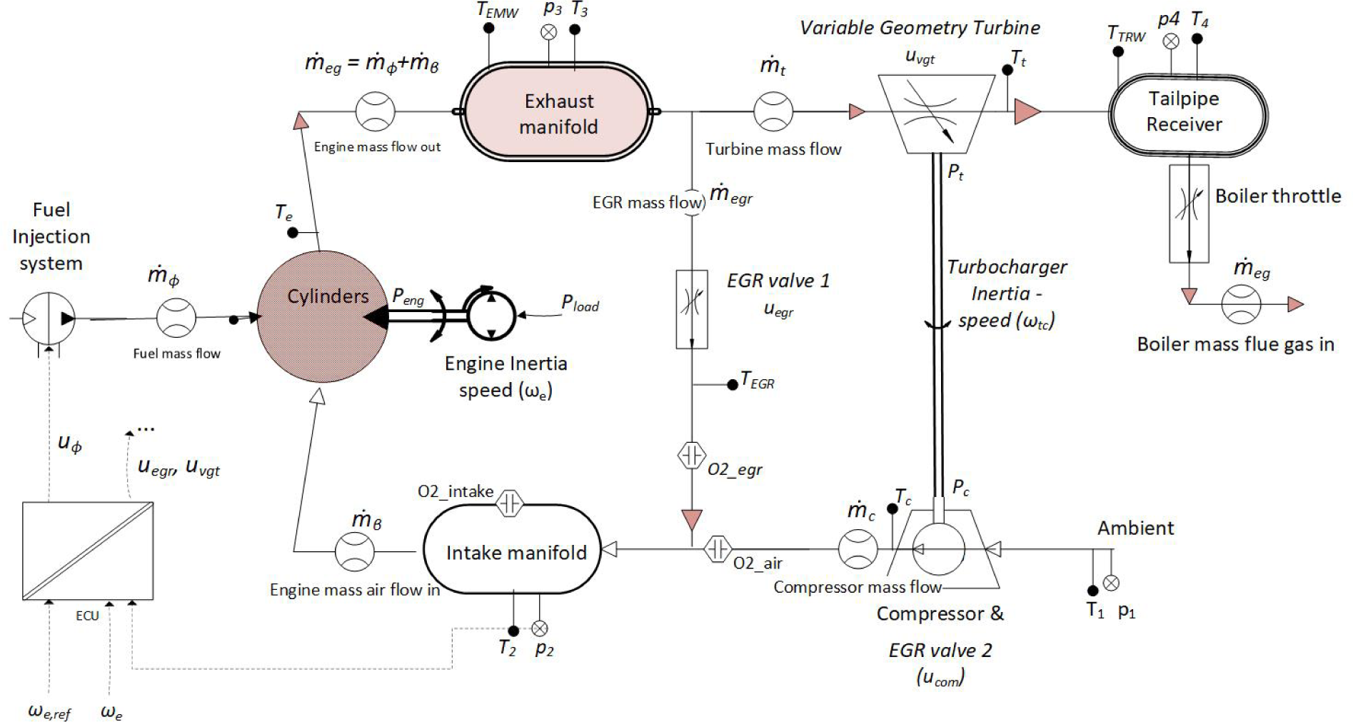
An overview of the typical system structure of a diesel engine is presented in Figure 4. The gas exchange system includes a turbocharger, cylinder as a volumetric pump, exhaust gas recirculation (EGR), and a variable geometry turbine. The fuel injection system, engine inertia, and turbocharger inertia are also present. The figure also indicates the input and output variables (input commands) used by the electronic control unit.
System structure of diesel engine
It is a resistance/flow component. A "compressor map" is the basis for compressor input-output calculation. The inputs to a compressor map are:
The pressure up-stream (p1) and down-stream (p2) of the compressor;
Compressor speed (ωtc);
Temperature upstream of the compressor (>T1>).
The outputs are:
Mass flow leaving compressor (ṁc);
Compressor efficiency (ηc), representing both isentropic efficiency and technical imperfections in the compressor realisation.
The power consumed by the compressor (Pc) to compress the gas (air) mass flow from its input to its output pressure level is:
(1)
in which is the pressure ratio over the compressor, and k = cp/cv where cp and cv are specific heats at constant pressure and constant volume, respectively.
The torque consumed by the compressor is:
(2)
The increased air temperature after compression is:
(3)
It is the first dynamic subsystem modelled as a reservoir/volume component [9]. The following ordinary differential equations (ODEs) describe pressure and gas temperature dynamics inside this receiver.
(4)
(5)
where VIR is the receiver volume. Note that this receiver has two inflows: air from the compressor and recirculated flue gas from EGR. Here the first law of thermodynamics for open systems is applied. It is assumed that no heat transfer through the walls is occurring, the fluids can be modelled as ideal gases, the specific heats for fresh air and flue gas are the same, and flowrates have a fixed, known direction.
It determines air (or mixture, in the case of EGR) mass inflow (ṁβ) and the combustion outputs, which are the torque generated by the engine and the temperature (Te) of flue gas at the outlet valve before entering the outlet receiver. The engine, modelled as a volumetric pump, transports air (or mixture) from the intake manifold to the outlet manifold. Air (or mixture) mass flow aspirated from the intake manifold into the cylinders is:
(6)
where is the gas density at the intake side, Vd is engine displacement volume, ωe is engine rotational speed, and N=2 for four-stroke engines (in every two rotations of the crankshaft, one full-cylinder gas volume is transported). The volumetric engine efficiency ηv indicates what portion of the full displacement volume is effectively used to pump the gas in and out the cylinders. This volumetric efficiency consists of two terms, one dependent on pressure ratio over the cylinders, and the other is a parabolic function of engine speed.
(7)
(8)
(9)
where cr is the engine's compression ratio, is the pressure ratio over cylinders, k is the ratio of specific heats, and are constant coefficients.
As an indirect input, it is a function of EGR valve opening (uegr) and the pressure ratio between intake and exhaust manifolds (Πe). For a control-oriented model, EGR mass flow is approximated by an orifice equation:
(10)
where is pressure ratio between intake and exhaust manifolds, cd,egr is discharge coefficient, and Aegr is the open area of the EGR valve. In addition:
(11)
Note that Aegr is a function of EGR valve opening. In the EGR pass, there might be a heat exchanger to cool down the EGR flow. EGR may also need a pumping device to create the required flow if the pressure on the exhaust side is lower than on the intake side.
The calculation starts with fuel mean effective pressure (pmf):
(12)
where Hl is the lower heating value of the fuel, and is the amount of fuel burned in each combustion cycle (consisting of four strokes).
The brake mean effective pressure pme is a portion of pmf determined by engine thermodynamic efficiency ηth minus total pressure losses (pml):
(13)
Total pressure loss includes losses by engine friction (pmlf) and gas exchange (pmlg):
(14)
For a diesel engine, pressure loss for gas exchange is the pressure difference over the cylinders:
(15)
Pressure loss by friction is modelled as a second order function of engine speed:
(16)
where apmlf1 and apmlf2 are constant coefficients.
Engine thermodynamic efficiency ηth consists of different terms dependent on engine speed, air-to-fuel ratio, and injection timing.
(17)
The speed-dependent efficiency term is a parabolic function of engine speed:
(18)
where ωe* is the speed with maximum efficiency and aη,th,ω is a constant coefficient.
The term dependent on air-to-fuel ratio is parametrised as:
(19)
where is the maximum value for this term, and and are non-negative constant coefficients.
The term dependent on injection timing is:
(20)
in which is the optimal start of injection angle and is a non-negative constant coefficient.
The engine torque finally is:
(21)
and mean engine power is:
(22)
When load power Pload acts on the engine, the ODE describing the engine speed dynamics is:
(23)
where is the engine's moment of inertia.
The mass flow that leaves the cylinders is the total of air mass inflow and fuel mass flow:
(24)
The balance of energy in the cylinders requires that the sum of the energy of input air (or mixture) and the combustion be equal to the sum of produced mechanical energy, heat losses to the coolant, and the energy that leaves the cylinders by the enthalpy of exhaust gas. This requirement gives the equation for exhaust gas temperature at the outlet valve:
(25)
in which kcool indicates how much of the available heat flux is carried by the exhaust gas. The coolant removes the remaining heat flux. The coefficient kcool is parameterised as:
(26)
where a0:2,cool are constant coefficients, and Me is engine torque. Coolant temperature may affect kcool especially in automotive applications when biofuel is used [36]; however, for stationary power generation kcool is assumed a function of engine torque.
It is another dynamic subsystem modelled as a reservoir/volume component. The following ordinary differential equations (ODEs) describe pressure and gas temperature dynamics inside this receiver.
(27)
(28)
where VOR is the exhaust receiver volume. Note that there are two outflows from this receiver, flue gas to turbine () and recirculated flue gas back to the intake receiver (). It is assumed that the fluids can be modelled as ideal gases, and flows have a fixed direction. Despite (convection/radiation) heat losses through the receiver walls are not considered for the intake manifold, these losses are quite significant on the exhaust side because of higher temperatures. Therefore, for the gas temperature dynamics inside the exhaust receiver, the heat losses from flue gas to the receiver wall () through convection are also modelled:
(29)
where and are the coefficient and surface area for convection losses.
An additional ODE is required to describe the dynamics of exhaust manifold wall temperature (). It is assumed that the heat transfer from the exhaust manifold wall to the ambient is only through radiation and is given by:
(30)
where is a coefficient for radiation heat transfer, and is ambient temperature.
The ODE for exhaust manifold wall temperature is:
(31)
When EGR is implemented, the states of the intake manifold and exhaust manifold are affected by EGR mass flow (). EGR also affects the dynamics of air-to-fuel ratio and oxygen availability in the engine flue gas. In the dynamic model of the EGR path, the intake and exhaust manifold states are represented by the mass of fresh air and recirculated flue gas in these reservoirs.
The ODEs for the mass of air and flue gas inside the intake manifold are:
(32)
(33)
where and are the contents of air in the intake and exhaust manifolds, respectively.
The ODEs for the mass of air and flue gas inside the exhaust manifold are:
(34)
(35)
In the above ODEs, is the amount of air needed for complete stoichiometric combustion of fuel mass flow , where is the stoichiometric air-to-fuel ratio.
Note that with this EGR model and perfect gas law, pressures inside manifolds (i.e., p2 and p3) are functions of their mass and temperatures.
The air-to-fuel ratio at the start of combustion is:
(36)
Assuming perfect mixing of gases inside the exhaust manifold, the weight content of oxygen in the engine flue gas is:
(37)
where MX is the molar weight of compound X.
Assuming CO2, H2O, N2 and O2 are the main flue gas species, the molar presence of H2O and CO2 in the flue gas from the complete combustion of FPBO is needed to calculate the molar oxygen content of flue gas. For oxygenated FPBO with averaged chemical formula CaHbOc, (e.g., C3.6H7.8O1.6), a complete FPBO combustion reaction reads:
(38)
Note that the averaged chemical formula is not referring to a real existing chemical compound of FPBO. It is based on the calculated average number of carbons, hydrogen, and oxygen atoms in one mole of FPBO. The published surrogate mixture of pyrolysis bio-oil is the basis for such calculation ([37]). Accordingly, the weight content of CO2 in the engine flue gas is:
(39)
and for H2O:
(40)
Then, the weight content of N2 in the engine flue gas is calculated by subtraction:
(41)
Finally, the molar content of oxygen in the engine flue gas is:
(42)
Turbine. It is a flow/resistance component. A "turbine map" is used for fluid-dynamic turbines to estimate their mass flow as a function of turbine pressure ratio and rotational speed. For a control-oriented model, turbine mass flow is approximated by an orifice equation:
(43)
where is pressure ratio over the turbine, is discharge coefficient, At is the open area of the turbine. In the case of a variable geometry turbine, cd and At are functions of turbine vane opening or nozzle area. The discharge coefficient is parameterised as a second-order function of turbocharger speed:
(44)
where are constant coefficients.
The power (or torque) generated by the turbine depends on its isentropic efficiency. In some control-oriented applications, turbine efficiency has been assumed constant. Experimental data are needed to model turbine efficiency as a function of pressure ratio, rotational speed, and nozzle area opening. Once turbine efficiency is modelled, the power generated by the turbine is:
(45)
where is turbine efficiency.
The torque generated by the turbine is:
(46)
The temperature of flue gas after the turbine is:
(47)
Friction is usually included in the turbine efficiency model. However, if efficiency is considered constant, then one could add a speed-dependent friction torque to the ODE of turbocharger speed:
(48)
where:
(49)
in which is a constant coefficient, is turbocharger friction torque, and is the turbocharger's moment of inertia.
The dynamics inside the tailpipe receiver are modelled similar to the exhaust manifold. The relevant state variables are p4 and T4 for pressure and temperature inside the receiver and TTRW - temperature of the tailpipe receiver wall. For the sake of brevity, the formulations of the ODEs are not presented here. Note that the ODEs of the tailpipe receiver require the estimation of mass flow out of this receiver (). This mass flow may be directed to the boiler burner or bypass the flue gas cleaning system through a valve/throttle. The backpressure created by the downstream components will determine the flue gas mass flow out of the valve/throttle.
NOx formation in a diesel engine is a function of torque generation, oxygen availability and engine speed. A mean-value model of the engine assumes all processes and effects are spread out over the engine cycle (4-stroke). Therefore, the mean-value NO concentration (cNO) is modelled statically by:
(50)
where p1, T1, and HM1 are pressure, temperature and humidity of intake air; Me, yO2,eg and ωe are engine torque, the oxygen content of flue gas, and engine rotational speed, respectively.
The boiler system consists of three components: a fuel injection system, combustion chamber, and heat exchanger. Fuel injection includes injection pump and injectors lifting. The combustion chamber model includes flame temperature, combustion reactions and the formation of pollutant emissions. The heat exchanger determines heat transfer from flue gas to water. The idea is to develop a detailed model to describe the transient short periods (start-up and cool-down). These periods are important for pollutant formation when the system should frequently respond to changes in the operating point of the upstream diesel engine (due to changes in power demand) and changes in hot water demands.
A first-order low-pass filter describes the dynamics of a fuel injection device. The parameters of such a model can be identified from experiments. The boiler/combustor system (combustion chamber and heat exchanger) involves some significant dynamics. Figure 5 presents a schematic view of the boiler/combustor system with its control-oriented input/output variables.
Schematic view of boiler components and input-output variables of the dynamic model
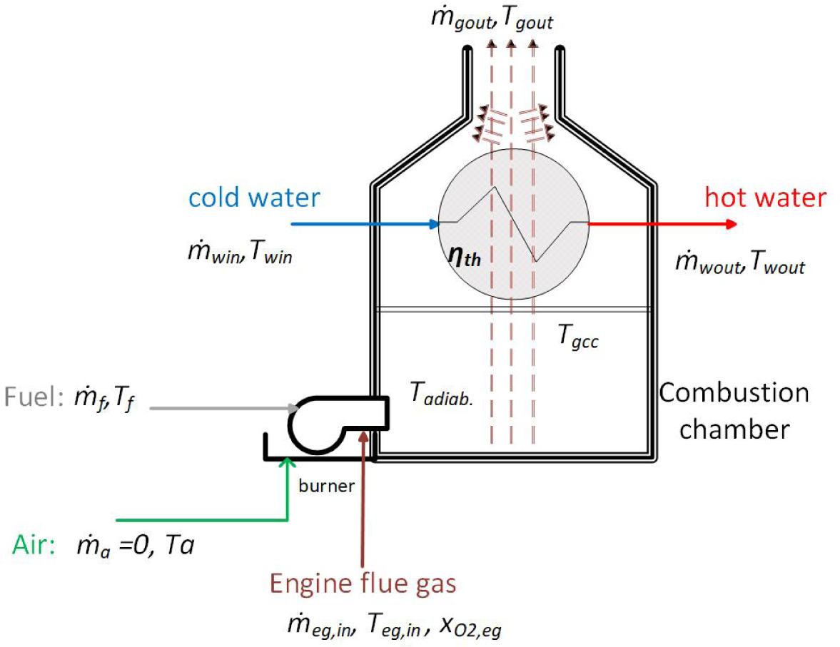
The following input, state and output variables are used in the presentation of the boiler dynamic model:
(51)
Assuming complete adiabatic combustion of FPBO in the boiler burner, the control-oriented boiler dynamic model starts with calculating the usable power on the gas side as:
(52)
in which is the useful power (amount of heat transferred from flue gas to water), is the heat generated by adiabatic combustion, - the heat flux into the system by the enthalpies of the three system inputs (air, fuel, and engine flue gas), ambient heat losses in the combustion chamber, and - the heat flux out of the system as the enthalpy of boiler flue gas. The formulations for these terms are as follows.
The heat generated by the adiabatic combustion is:
(53)
where is specific enthalpy of gas flowing in the combustion chamber.
The sum of input enthalpies reads:
(54)
The total energy input to the combustion chamber is the sum of the heat generated by the combustion and input enthalpies. Therefore, the enthalpy of gas in the combustion chamber is:
(55)
Ambient heat losses in the combustion chamber and burner box are assumed proportional to the heat input to the combustion chamber.
(56)
where is the heat loss coefficient. This term refers to heat losses through convection and radiation, parameterised by a third-order polynomial of .
(57)
Heat flux out of the boiler chimney by the enthalpy of flue gas is:
(58)
where is steady-state temperature of flue gas out of the boiler chimney.
Boiler thermal efficiency is defined by:
(59)
Thermal efficiency is parameterised as a function of boiler operating point (represented by ):
(60)
Then is calculated as:
(61)
When assuming perfect gases with constant , the specific enthalpies expand as:
(62)
Two thermal reservoirs exist in the boiler model: thermal capacity of water (including its piping) and thermal capacity of flue gas, mainly due to the mass of flue gas tubes. Two ODEs describe the dynamics of these reservoir temperatures [11].
Assuming a lumped parameter model for the water subsystem, i.e., fixed volume water reservoir with homogeneous temperature all over the reservoir and a constant water flow rate and temperature, the ODE for the temperature of water in the reservoir reads:
(63)
where Cw is the thermal capacity of the water reservoir (water+piping) and cp,w is the specific heat of the water.
The dynamics of flue gas temperature out of the boiler (at the chimney) are described by the following ODE:
(64)
where Cg is the thermal capacity of flue gas reservoir (e.g. metal tubes) and cp,g is the specific heat of flue gas.
Sub-model of the oxygen content in the flue gas. A general chemical formula for FPBO and its complete combustion reaction (with fresh air) reads:
(65)
When the flue gas from the engine is used as an oxidiser in the boiler burner, the reaction for complete combustion reads:
(66)
Oxygen available for the burner flame temperature is the sum of the oxygen content of flue gas and oxygen from fresh air, if any. It should be noted that although in this boiler dynamic model, the fresh air inflow is considered as an input, it is not meant to be present in the final design of the boiler system. Obviously, one can eliminate the fresh air element from the model but it is present in the model for the sake of model generality and flexibility.
Oxygen mass flow present in the fresh air is:
(67)
where the molar oxygen content of fresh air is 21%. Assuming CO2, H2O, N2 and O2 to be the main species of flue gas, and when the oxygen content of flue gas is , then the mass flow of oxygen present in the flue gas is:
(68)
Note that the molar contents of CO2, H2O, and N2 in the flue gas are dependent on FPBO chemical formula and oxygen content of flue gas. The total available oxygen mass flow is:
(69)
When an FPBO-fuelled flue gas burner uses the oxygen in engine flue gas as an oxidiser and the air-to-fuel ratio is constant, NOx formation in such a burner is a multiple linear function of engine flue gas temperature and oxygen availability [38]:
(70)
where , i = 0, 1, 2 are the constant coefficients of the multiple linear regression model.
The adiabatic flame temperature at constant pressure Tadiab is a function of inputs, particularly the oxidiser/fuel ratio. When engine exhaust gas is used as an oxidiser, the equivalent oxidiser-to-fuel ratio is:
(71)
where is the stoichiometric oxidiser/fuel ratio. The only oxidiser in the SmartCHP boiler system is the engine flue gas. Obviously, the equivalent oxidiser-to-fuel ratio depends on the oxygen content of the engine flue gas.
Assuming complete combustion of FPBO in the burner and a lean oxidiser/fuel mixture, the balance of energy before and after combustion requires:
(72)
where Hl is the lower heating value of FPBO. In a lean mixture, the equivalent oxidiser-to-fuel ratio is greater than unity . When a mixture of air and engine exhaust gas is used as an oxidiser, then we have:
(73)
and the balance of energy leads to:
(74)
In a rich mixture of oxidiser/fuel , however, the available oxidiser amount determines the combustion rate, and the balance of energy before and after combustion requires:
(75)
which leads to:
(76)
Figure 6 depicts an SCR unit with its injection device. The SCR gas treatment will require urea/ammonia as its reducing agent.
Schematic view of Selective Catalytic Reduction with its injection device
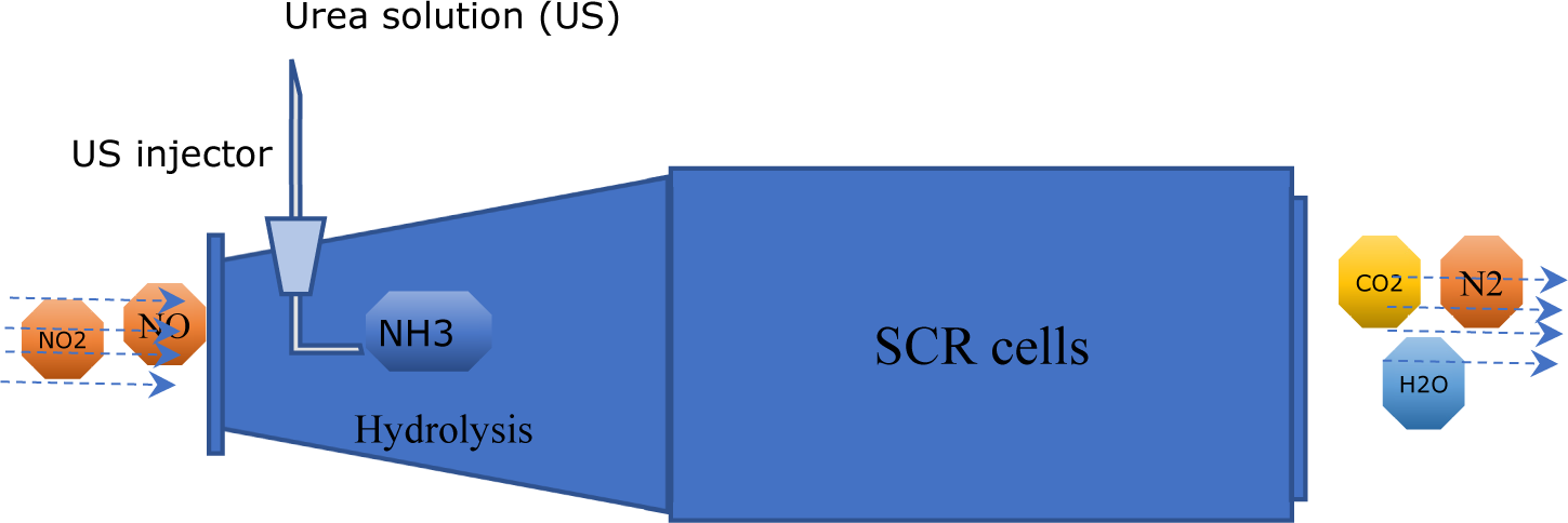
A complete control-oriented model of the SCR system includes the dynamics of the urea solution injection device, the decomposition (hydrolysis) of water-urea solution into gaseous ammonia and CO2, the reducing chemical reactions, and the dynamics of the NOx/NH3 sensor. A first-order low-pass filter could represent the dynamics of the urea injection device. One can identify the parameters of such a model from experiments. The NOx/NH3 sensor dynamics depend on the sensor's type and quality. An ideal perfect NOx sensor gives a direct and accurate measurement of NOx. An actual sensor measurement, however, may be corrupted by cross-sensitivity to NH3. The output of the such sensor may require some filtering before it is used for control design.
The assumptions for the control-oriented model of hydrolysis reactor are the following:
The water-urea mixture is at ambient temperature before injection and will be heated up to the temperature of the hydrolysis reactor after injection (perfect mixing).
The decomposition of urea solution into gaseous ammonia is very fast and is modelled statically.
The flue gas temperature out of the hydrolysis section is the same as that of the hydrolysis reactor (lumped parameter).
No heat losses to the ambient are considered as these are included in the thermal model of SCR cells.
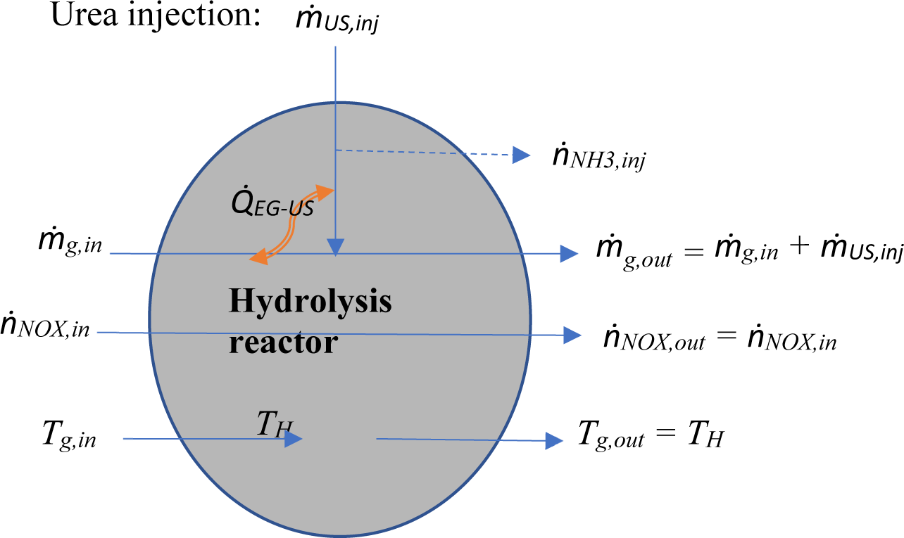
Figure 7 shows the hydrolysis reactor's mass and heat flow in/within/out. The ODE for the temperature inside the reactor (TH) is:
(77)
where is the thermal capacity of the hydrolysis reactor considering specific heat capacity and mass .
is the heat transferred from flue gas to urea solution. This heat is consumed for water boiling, vaporising, and heating of water/urea vapour to the temperature of hydrolysis reactor.
(78)
where and are specific heat capacity of liquid water and water vapour, respectively, is specific heat capacity of urea, and is specific heat of water vaporisation.
mass and heat flow in/out of hydrolysis reactor
Variables and are the mass flows of water and urea:
(79)
(80)
where denotes urea concentration in the water-urea mixture.
The molar flow of NH3 into the SCR cell is calculated statically as a function of urea solution mass injected:
(81)
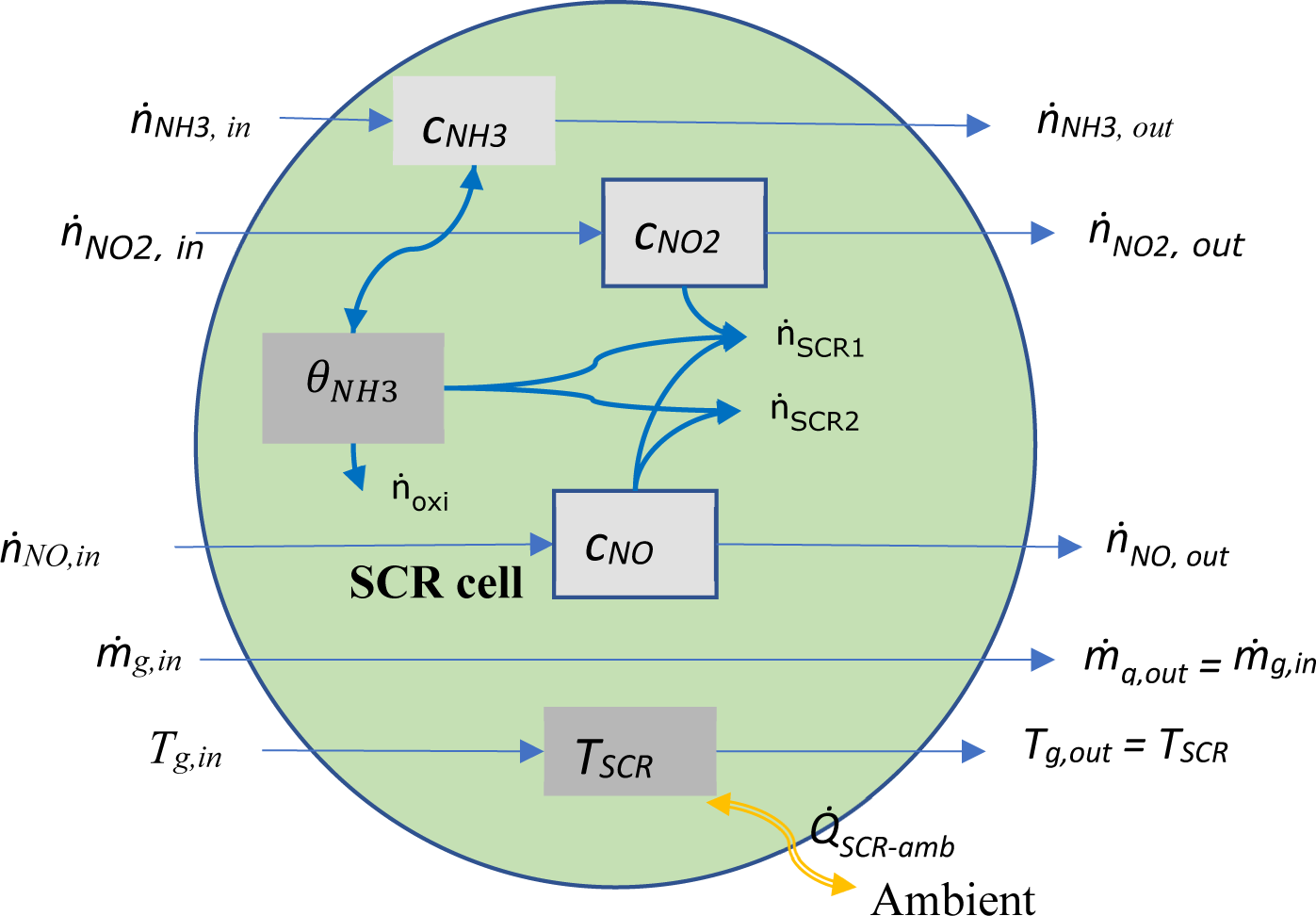
SCR is a continuous system in which the concentration of its species (NH3 and NOx) changes continuously along its length. However, for its control-oriented modelling, the SCR unit is usually discretised into 2 or 3 cells; inside each cell, the concentrations can be assumed homogeneous. This approximation is a control-oriented practice and might not be regarded proper for other applications. The main dynamics of an SCR cell relate to its reducing chemical reactions. [Figure 8] shows a control-oriented representation of an SCR cell and its inputs-outputs. The chemical reactions included in this representation are adsorption and desorption of ammonia on the catalyst's surface, the fast SCR reaction using equimolar amounts of NO and NO2, the main SCR reaction, and the oxidation of adsorbed ammonia from the surface of the catalyst.
The reaction for adsorption and desorption of ammonia on the catalyst reads:
The forward reaction rate of adsorption (rads) is proportional to gaseous ammonia concentration (cNH3) and the remaining capacity for adsorption (1 − θNH3) on the catalyst surface:
(82)
Mass and heat flow in/out of SCR cell
The backward reaction rate of desorption (rdes) is proportional to the used capacity for adsorption:
(83)
where is the scaled surface coverage with ammonia, cS – the concentration of active surface atoms per gas volume, SC − the area of one mole of active surface atoms, αpr − the sticking probability, MNH3 − the molar mass of ammonia, kdes − pre-exponential factor desorption, and Ea,des is the activation energy of desorption.
The fast SCR reaction (SCR1) using equimolar amounts of NO and NO2 reads:
Its rate is proportional to the available adsorbed ammonia and the minimum of NO and NO2 concentrations:
(84)
where kSCR1 is the pre-exponential factor, and Ea,SCR1 is the activation energy of SCR1.
The main SCR reaction (SCR2) with NO only reads:
The rate of reaction is proportional to the available adsorbed ammonia and the minimum of NO and O2 concentrations:
(85)
where kSCR2 is the pre-exponential factor, and Ea,SCR2 is the activation energy of SCR2.
The oxidation of adsorbed ammonia reads:
Its reaction rate is:
(86)
where kox is the pre-exponential oxidation factor, and Ea,ox is the activation energy of oxidation. Note that in lean conditions, where enough oxygen is available, only NO and NH3 concentrations become important for calculating rSCR2 and rox. All the reaction rates are given in [].
The concentration of gases in the SCR may not be uniformly distributed. Therefore, their dynamics should be expressed by partial differential equations. However, suppose the SCR is divided into a few cells arranged in series. In that case, uniform gas concentration distribution and homogeneous temperature in each cell is a justifiable (lumped parameter) assumption for an acceptable approximation of the dynamics. With this approximation, a set of ODEs can represent the dynamics in each cell.
The ODE for the concentration of ammonia reads:
(87)
where is the volume of each cell, as SCR volume Vc is divided into ncell cells, and is the flue gas volume flow out of the SCR cell. The first term on the right-hand side of this ODE is the rate of ammonia concentration change by the ammonia inflow, the second term is the rate of concentration change because of gas outflow, and the last two terms are the rate of adsorption and desorption, respectively. The volume flow rate is:
(88)
where pamb denotes ambient pressure.
Similarly, the ODE for NO concentration is:
(89)
and the ODE for the concentration of NO2 reads:
(90)
One can express the dynamics of adsorbed ammonia on the catalyst surface by:
(91)
Considering the SCR cell and its housing as a thermal reservoir, its temperature dynamics can be expressed by:
(92)
where is the thermal capacity of SCR cell, with specific heat capacity cp,SCR and mass (SCR mass divided by the number of cells). The heat radiated and transported by convection from the SCR cell to its ambient is:
(93)
where and are the coefficient and surface area for heat transfer by radiation/convection.
The molar flow of the gas out of the SCR cell is calculated as a function of the cell state variables:
(94)
where i is the index for species NH3, NO, and NO2.
The following assumptions have contributed to the simplification of the SCR dynamic model:
The urea decomposition is fast and occurs completely before entering the first SCR cell. Therefore, the molar flow of ammonia into the first SCR cell is a static function of molar urea injection.
Reaction enthalpies and their thermal effects are neglected.
More simplifications of the SCR model derive from only considering NOx and ammonia concentrations in their steady state. This assumption is acceptable because their dynamics are much faster than the dynamics of thermal energy storage and NH3 adsorption on the catalyst's surface [8].
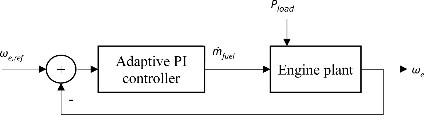
For parameter optimisation of the engine model, an adaptive PI controller with the structure shown in [Figure 9] simulates the performance of the engine speed governor. This controller estimates the change in electrical load on the diesel engine and regulates the fuel injection accordingly.
Structure of control strategy for engine speed governor
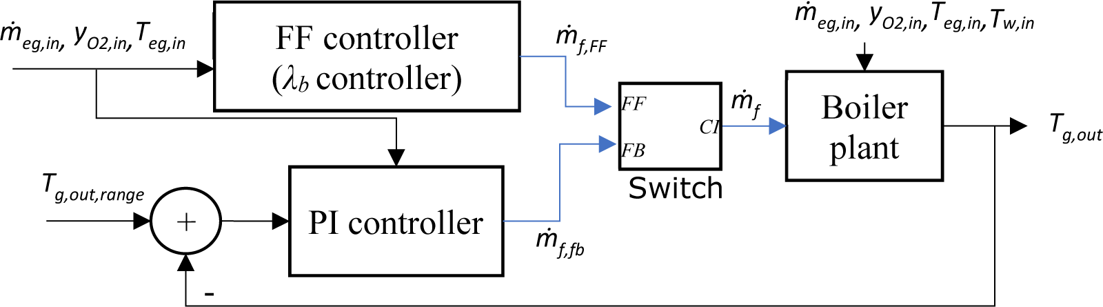
As a defined operating condition, the boiler flue gas temperature should be kept between 230−550 °C to minimise harm to the downstream cleaning system. [Figure 10] shows a control strategy for the temperature of boiler flue gas, formulated based on the dynamic model described in the previous section. This strategy exploits switching between feed-forward (FF) control of oxidiser-to-fuel ratio and feedback control of boiler flue gas temperature. The FF controller regulates the fuel rate to keep the oxidiser-to-fuel ratio constant at a predefined reference value to ensure optimal combustion of FPBO in the combustor and better fuel efficiency. However, when the flue gas temperature exceeds/falls below the maximum/minimum temperature allowed, the PI controller decreases/increases the fuel rate to push the temperature back to its acceptable interval. This feedback action will compensate for the oxidiser-to-fuel ratio from its reference value. In the simulations presented in this paper, the feedback controller is switched off, and only the oxidiser-to-fuel ratio is controlled because the experimental setting used to tune burner parameters is air ratio-controlled only.
Structure of control strategy for boiler flue gas temperature and oxidiser-to-fuel ratio
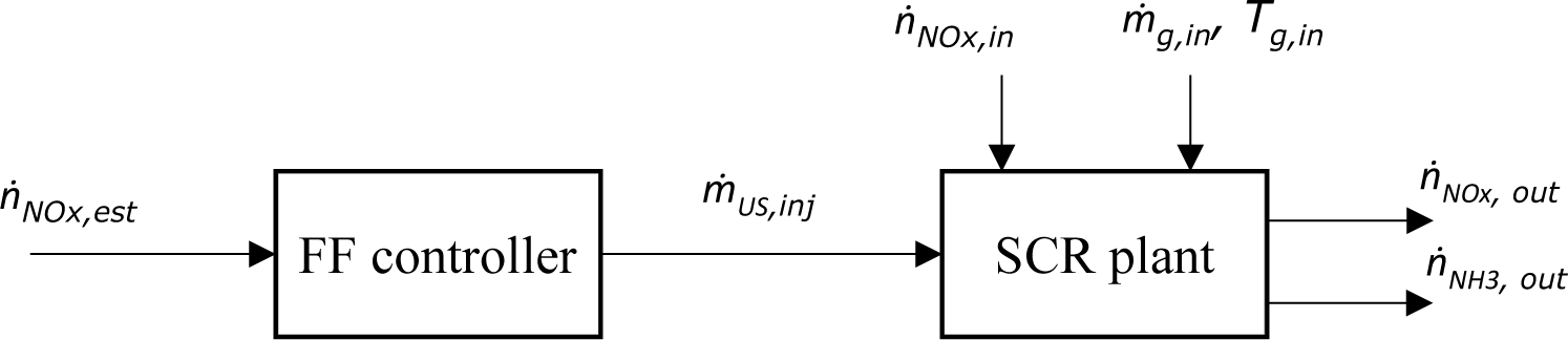
One can use both feed-forward and feedback controllers for optimal NOx removal. [Figure 11] shows the structure of a feed-forward control strategy is shown in. In this control design, the molar flow of NOx is estimated as a function of upstream plants (engine + boiler) operating point. For example, NOx formation for the engine is a function of engine torque and rotational speed. NOx formation for the burner is a function of flue gas temperature entering the burner and its oxygen content. The controller calculates the amount of urea solution injection for the estimated NOx molar flow.
Structure of control strategy for NOx removal by SCR
As the SmartCHP plant is under construction and experimental validation of its model is not possible at this stage, data from individual components are the basis for tuning their parameters. For parameter tuning, we have formulated nonlinear regression models to minimise the error between predictions by the model and the available experimental data.
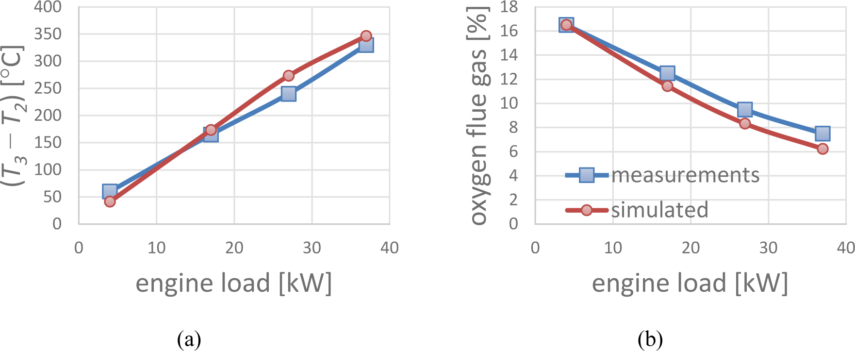
The parameters of the diesel engine model are tuned to steady state measurements of compressor mass flow, flue gas oxygen, turbo pressure, and after-turbine flue gas temperature from an experimental diesel engine running on FPBO blend with methanol [39]. For more on the experimental setup, refer to [40]. The engine runs at different load steps (4−17−27−37−47 kWe) with a constant engine speed of 1500 rpm. [Figure 12] compares engine measurements with model predictions.
Comparison of engine measurements and model prediction: flue gas temperature raising around the cylinder (a); oxygen content of engine flue gas (b)
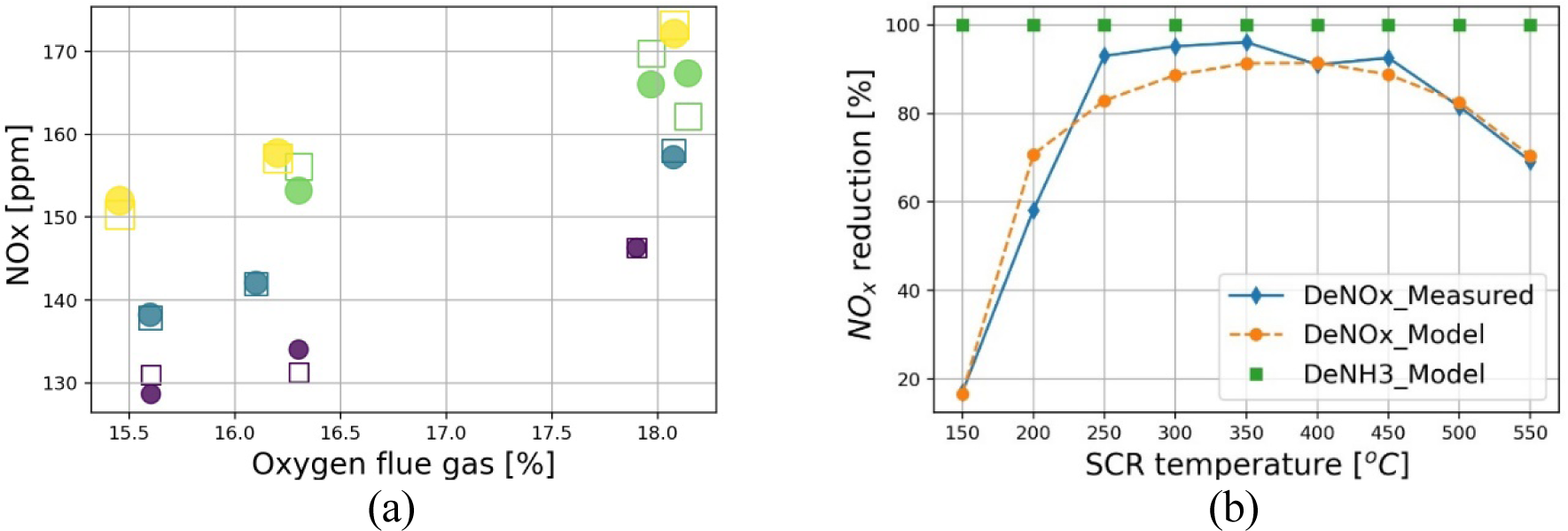
Data from an experimental setup of burner/boiler running on FPBO with artificial engine flue gas as oxidiser [38] are used to parameterise the model of NOx emissions from burner/boiler. In the experiments, the input flow to the burner is a mixture of air, nitrogen, and carbon dioxide. The oxygen content of the inflow mixture and its temperature are adjusted by regulating mixture percentages and mixture preheating, respectively. [Figure 13a] compares measurements of burner NOx emission with the model predictions. Oxygen content varies between 15−19%, and inflow temperature between 200−450 oC.
Comparison of model prediction with experimental data: NOx emissions from the burner at a variable oxygen content of flue gas − square hollow markers show experimental data and circle filled markers show model data, the colours show different flue gas input temperatures (a); NOx reduction by SCR at different SCR temperatures (b)
For the DPF backpressure model, the data in [13] are used where experimental measurements of volume flow rates of exhaust gas, particulate mass, and inlet exhaust temperatures are available. For OC model parameter tuning and estimation of its effect on NO/NO2 ratio, the data in [41] and [42] are used. In the experiments, an OC unit is mounted for after-treatment of exhaust gas from a 4-stroke, 4-cylinder diesel engine. The experimental setup was equipped with a non-dispersive ultraviolet analyser to measure nitric oxide (NO) and nitrogen dioxide (NO2) separately.
The data used for SCR parameter tuning are from Kwak et al. [43], where model Cu/zeolite catalysts were experimentally investigated, and their NOx reduction performance at different SCR temperatures was recorded. [Figure 13b] compares NOx reduction performance by the SCR model and those reported by Kwak et al. [43]. The mean absolute percentage error is 5.9%. The figure also shows NH3 reduction percentages predicted by the model.
In this section, first, we show how power and heat generation are nonlinearly coupled. Then the simulation results and the controllers' evaluation are given for power-led mode. Some more common operating modes of micro-CHPs are power-led, heat-led, or economy modes. In a power-led mode, there is one degree of freedom, and that is to follow the power demand profile. In a heat-led mode, priority is given to fulfilling the heat demand; however, SmartCHP has a nonlinear power and heat generation coupling. An optimisation problem needs to be formulated to follow the heat demand and then, with the remaining degree of freedom, to follow power demand, minimise emissions, or maximise efficiencies. In an economy mode, priority is given to cost minimisation, profit maximisation, minimum emissions, or maximum efficiency. Neither heat demand nor power demand will be followed completely. Problem formulations for heat-led and economy modes and their solution methods are beyond the scope of this paper. They are further steps towards implementing a smart control unit for the cogeneration unit. Future research will address the mentioned optimisation problems.
From equation (36), the fuel mass flow that can be injected into the burner/boiler is:
(95)
The heat generated from the boiler is:
(96)
The heat input by engine flue gas into the boiler is:
(97)
where is the share of heat exhausted from the engine in flue gas, parameterised in (26).
Useful heat from flue gas from boiler and CHP engine reads:
(98)
where is the thermal efficiency of heat recovery from the exhaust gas, and is the heat loss coefficient from the boiler burner box and combustion chamber.
Useful heat recovered by the engine coolant is:
(99)
where is the thermal efficiency of heat recovery by the engine coolant.
Total useful heat is:
(100)
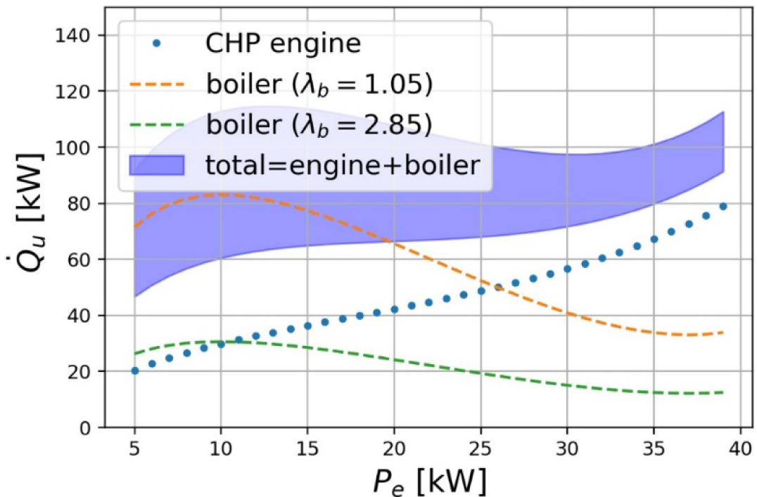
[Figure 14] shows total useful heat generation and heat generation from the operation of individual components, i.e., engine and boiler, as functions of engine power. Heat generation from the boiler can be controlled by adjusting the boiler oxidiser-to-fuel ratio () in a feasible range 1.05−2.85 where minimum gives maximum boiler heat generation. This plot suggests that heat and power generation will not completely be decoupled in the SmartCHP concept. At engine power of around 10−15 kW, maximum heat generation becomes possible. Every point in the blue highlighted area is possible for power/heat generation. This plot shows that the feasible operation region area of the SmartCHP system is considerably larger (i.e., more than 100%) than that of the CHP engine. Hence, there is a certain degree of freedom for heat generation at all the engine operating points, which can be exploited for optimisation when the plant is operated in heat-led mode.
Heat generation as a function of engine power
In this section, the response of the SmartCHP plant to fluctuating load demand is predicted, i.e., in power-led mode. The primary driving parameter in simulations is the electrical load on the modified diesel engine. In the simulated scenario, the load demand profile is based on promising use cases (e.g., hospitals) for SmartCHP in connection with the market assessment [44]. The load on the diesel engine starts with a minimum of 12 kW for 5 h, then ramps up to 40 kW in one hour, and in the next 14 h, it slowly decreases to 15 kW and stays there for the rest of the day. It is assumed that heat demand is constant at 58 kW for all the hours. Simulations will show at which hours the heat from the CHP engine is not enough to respond to this heat demand thereby, and the boiler should generate extra heat. Conversely, there will be times when the heat from the CHP engine exceeds heat demand; thereby boiler should be off. We adjust system time constants for a reasonable simulation run time so that every hour shrinks to 200 s of simulation time.
Flexibility, low emission and high fuel efficiency at all power levels are the motivations for SmartCHP. Therefore, in this section, predictive simulations show the results of heat-to-power ratio, energy production, energy efficiencies, and NOx emissions. Moreover, the performance of the controllers is evaluated. The formation of NOx and the performance of SCR in reducing this pollutant are depicted. Dynamics of pressure, temperature, mass flow, and oxygen content of flue gas at different plant sections are also shown.
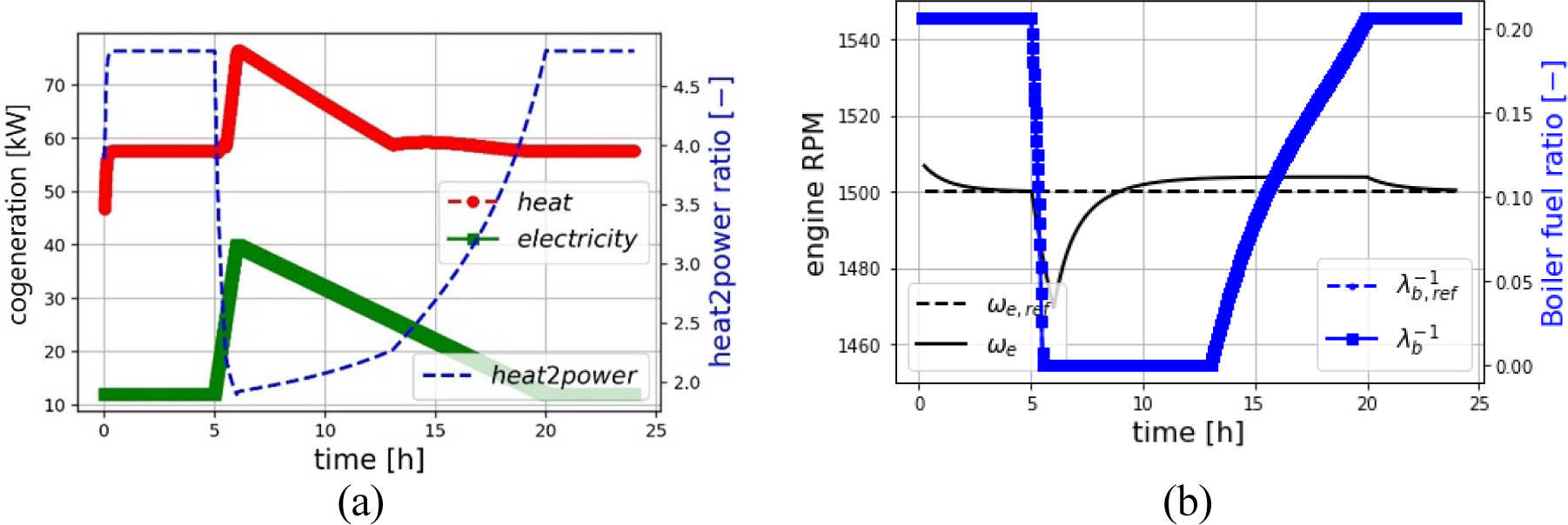
As the engine load in [Figure 15a] increases, more heat becomes available through the engine jacket and its flue gas heat recovery. When engine load decreases, the temperature of its flue gas drops but its oxygen content increases. This trend allows the boiler to bear more heat load, thereby maintaining the response to the high heat demand. In this mode of operation, the plant offers a wide range of heat-to-power ratios, as shown in [Figure 15a]. One can derive plant machine utilisation rates from these figures.
[Figure 15b] shows the performance of the preliminary controllers. Engine governor design allows for satisfactory constant speed control. The burner oxidiser-to-fuel ratio controller is a feed-forward type that uses estimated values of engine flue gas temperature and composition (mass flow and oxygen content) for regulating fuel injection. This controller reaction may fall behind engine flue gas changes at high engine transient. Nevertheless, the controller shows a good performance in reference tracking. [Figure 15b] depicts the inverse of oxidiser-to-fuel ratio (i.e., fuel ratio); when it is zero, it means the boiler is off.
Power-led response to a typical hospital electricity demand profile: heat and power generation (a); engine rotational speed and burner oxidiser-to-fuel ratio control (b)
One can perform the efficiency analysis using energy or exergy concepts [45]. [Figure 16a] presents the energy efficiencies calculated as the ratio of output useful energy to input energy of FPBO with a low heating value (LHV) of 16.9 MJ/kg [46]. The assumptions are the following:
thermal efficiency of heat recovery from engine cylinder by the coolant is 60%,
thermal loss from the boiler combustion chamber and burner box is 2%,
40% of flue gas heat is consumed for water heating in the boiler while the rest goes to the cleaning system; this number depends on tubes sizes in the boiler heat exchanger,
thermal efficiency of heat recovery from exhaust gas downstream of SCR is 95%.
Power-led response to a typical hospital electricity demand profile: in energy efficiencies (a); in NOx formation (b)
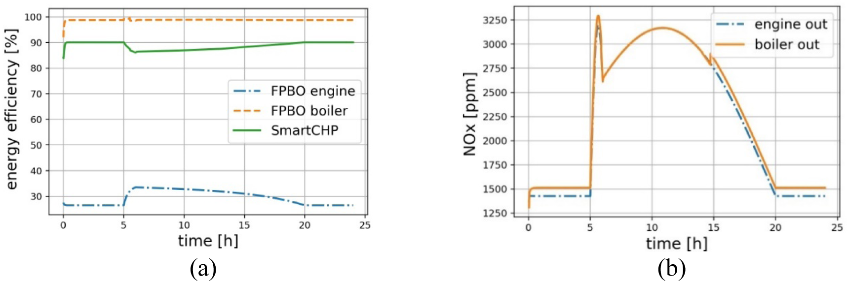
The efficiency of electricity generation can increase to 33% at full load, but at low engine load, the fuel efficiency of electricity generation is low. The simulations after a time of 50 s show that plant can maintain overall fuel efficiency of at least 80% at both low and high engine loads. Boiler energy efficiency also remains high at different engine loads. Note that engine flue gas enthalpy is an energy input to the boiler system, and the assumption for the calculation of boiler energy efficiency is that a high-efficiency heat recovery system is in place downstream of the boiler to recover heat from the boiler exhaust gas. Moreover, boiler energy efficiency at engine transients might hit higher efficiencies than 98% because a large heat capacity of the boiler heat exchanger can, for a short while, keep providing input energy to heating water after transient of engine flue gas. Notably, final efficiency analysis of the cogeneration plant is possible when realistic heat-recovery efficiencies are provided and input parameters are optimised (see, for example, [47]).
[Figure 16b] depicts the formation of NOx in the engine flue gas and boiler flue gas. Most of the NOx is due to engine operation, while the boiler has a minor contribution. At high engine loads, NOx formation can reach above 3000 ppm.
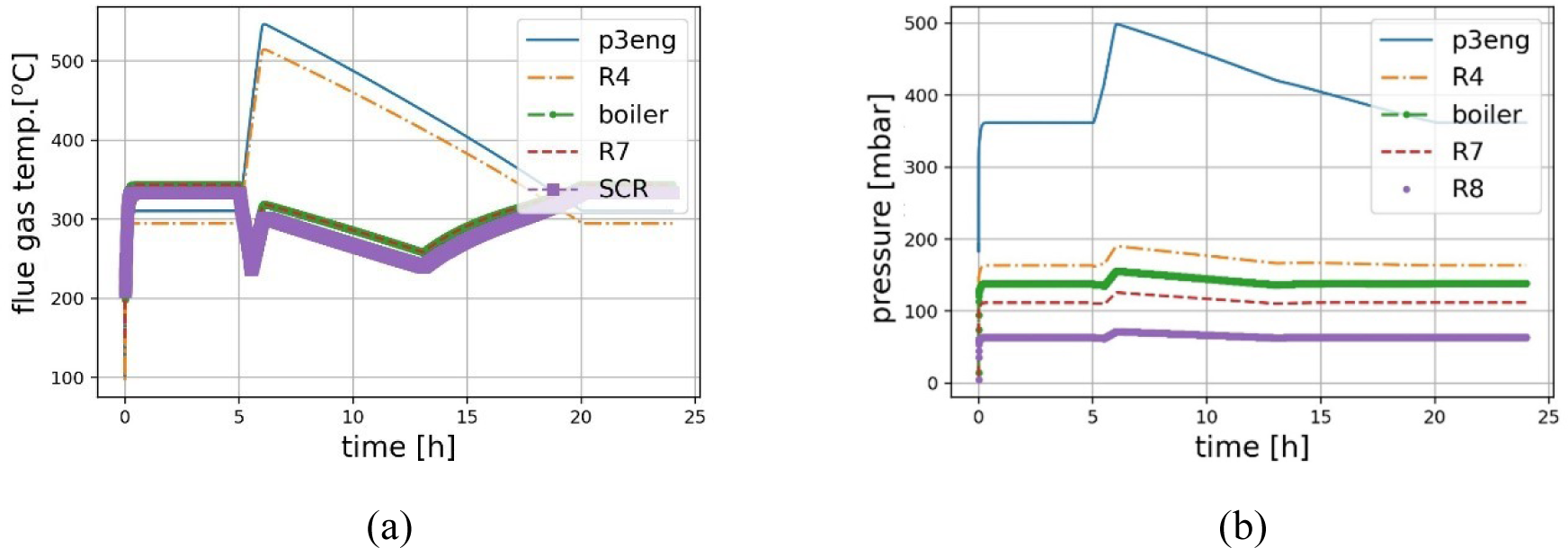
The evolution of flue gas temperature at different sections of the plant is shown in [Figure 17a]. For an electrical load change from 12 kW to 45 kW, the flue gas temperature at engine exhaust (p3eng) and tailpipe reservoir R4 (before entering the boiler burner) increases from 300 to 530 oC. However, flue gas temperature at boiler exhaust pipe undergoes an opposite trend, with less amplitude of fluctuations (250−340 oC). When the boiler is off (between hours 5−13), the big gap between the temperature of flue gas at the engine outlet and the boiler outlet indicates the heat release to water in the boiler exchanger. After hour 13, the boiler is on again to cover the heat demand and its flue gas temperature rises.
[Figure 17b] shows how flue gas pressure increases as diesel engine load increases. Spatially, the pressure decreases as the flue gas goes through the boiler and finds its way through the cleaning system. Every part of the cleaning system acts as a flow restriction and might contribute to pressure drop. Diesel particulate filter, due to soot accumulation, is a component causing a significant portion of this pressure drop.
Power-led responses to a typical hospital electricity demand profile at different plant sections: flue gas temperature (a); flue gas pressure (b)
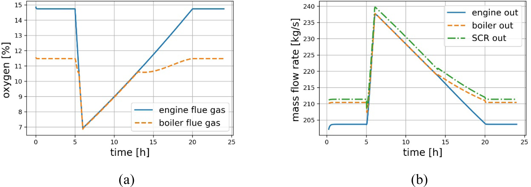
As engine load increases/decreases, its oxygen content drops/goes high ([Figure 18a]). Mass flow rate is also almost proportional to engine load ([Figure 18b]). The increment of boiler mass flow out relative to engine mass flow out is the extra FPBO injected into the burner. The mass of urea solution injected upstream of SCR is the difference between boiler and SCR outflows. The flue gas boiler's response to the oxygen content change also depends on heat demand. When there is enough oxygen and some heat is needed, the boiler will use the available oxygen to generate more heat; otherwise, it remains off.
Power-led responses to a typical hospital electricity demand profile at different plant sections: oxygen content in flue gas (a); mass flow rate of flue gas (b)
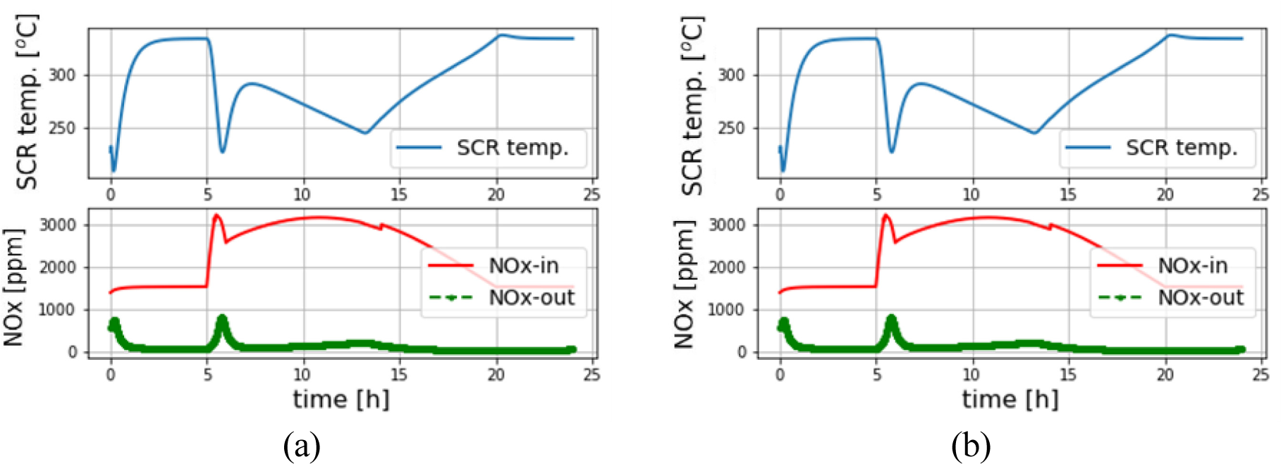
The performance of SCR NOx reduction with a feed-forward controller is illustrated in [Figure 19a] and [Figure 19b]. Here the SCR plant is modelled by two SCR cells. A step change in the estimated NOx excites the controller to increase urea injection. Two scenarios consider the effect of SCR temperature on NOx reduction. In the first scenario, shown in [Figure 19a], 40% of flue gas heat is consumed for boiler water heating. As a result, the SCR temperature stays above 220 oC. The controller can keep NOx emission low (below 500 ppm), especially in steady state operation, but in fast transients (time slot between hours 5 and 6), there is a peak in NOx leak downstream SCR. Here, controller performance needs improvement, for instance, by adding a feedback component to respond to a sudden increase in NOx formation. Further controller design optimisation will be pursued when experimental data from the developed cleaning system of SmartCHP become available.
In the second scenario, shown in [Figure 19a], 60% of flue gas heat is consumed for boiler water heating which leads to cooler SCR temperature (below 230 oC). Here, a cool converter severely degrades the performance of NOx reduction. The degraded performance of SCR in cool temperatures below 230 oC agrees with data published in the literature, e.g., see [Figure 13b]. This scenario points to a potential design issue normally addressed in the design phase of the boiler heat exchanger. Nonetheless, one must avoid such a cool SCR situation during normal plant operation to keep emissions within limits.
NOx reduction performance when water heating in the boiler consumes, of the flue gas heat: 40% (a); 60% (b)
A control-oriented dynamic model of a newly designed cogeneration plant fuelled with fast-pyrolysis bio-oil was presented. The cogeneration plant includes a modified diesel engine operating on FPBO, a newly designed flue gas burner that oxidises FPBO only with the oxygen content of engine flue gas, and a dedicated flue gas treatment system to remove CO, HC, and NOx. According to the literature review of the existing dynamic models, no dynamic model could be directly used or fit for predictive simulation of this plant. Furthermore, FPBO is the new fuel for diesel engines and swirl burners, and the hybrid operation of the engine and boiler implies a semi-decoupled cogeneration concept. These aspects have necessitated new dynamic modelling at both the components and system levels. The plant model also integrates dynamic models of heat exchangers, condensers, tailpipe gas reservoirs, and injection devices. Predictive simulations show the potential of this plant for flexible heat/power ratio generation and its potential to respond to energy demands for a wide range of engine loads while maintaining overall energy efficiency above 85%. The performance of the control design was evaluated on the component level through dynamic simulations. Results showed the need for an advanced cleaning system control design when fast transients cause a sudden increase in NOx formation. Control design should also address keeping SCR temperature at a certain range to ensure maximum NOx reduction.
The industrial application of the proposed plant model can be in three areas. A dynamic model can be used to evaluate the operating conditions of the components at different operating modes and to find optimal working conditions. The proposed model is a tool to perform predictive simulations, evaluate component controllers' performance, and identify areas where advanced controllers are needed. The dynamic model generates input parameters, i.e., the plant's machines' utilisation rates, efficiencies, and emissions in response to a user load profile and usage preferences which are input parameters for energy cost models and feasibility studies.
The current integrated system model is based on the integration of individual models of system components, validated individually. However, validation of the system model with data from the integrated plant is yet to be performed when a prototype of the integrated system is completed and the operation data become available. The simulation results are presented only for the power-led operating mode. Based on the proposed dynamic model, formulation of optimisation problems and their solution methods to derive the best working points in heat-led and economy modes remain for future research.
The SmartCHP project has received funding from the European Union's Horizon 2020 Research and Innovation Programme under Grant Agreement No. 815259. The authors would like to thank the SmartCHP project partners for the interesting discussions and provision of experimental data.
- ,
Potential contribution of biomass to the sustainable energy development ,Energy Convers. Manag , Vol. 50 (7),pp 1746-1760 , 2009, https://doi.org/https://doi.org/10.1016/j.enconman.2009.03.013 - ,
Opportunities for biomass-derived 'bio-oil' in European heat and power markets ,Energy Policy , Vol. 34 (17),pp 2871-2880 , 2006, https://doi.org/https://doi.org/10.1016/j.enpol.2005.05.005 - ,
Optimisation of biomass-fired cogeneration plants using ORC technology ,Renew. Energy , Vol. 159 ,pp 195-214 , 2020, https://doi.org/https://doi.org/10.1016/j.renene.2020.05.155 - ,
Energy, exergy and exergoenvironmental analyses of a sugarcane bagasse power cogeneration system ,Energy Convers. Manag , Vol. 222 (113232), 2020, https://doi.org/https://doi.org/10.1016/j.enconman.2020.113232 - ,
Simulation-based strategies for smart demand response ,J. Sustain. Dev. Energy, Water Environ. Syst , Vol. 6 (1),pp 33-46 , 2018, https://doi.org/https://doi.org/10.13044/j.sdewes.d5.0168 - ,
Modelling and control of collecting solar energy for heating houses in Norway ,J. Sustain. Dev. Energy, Water Environ. Syst , Vol. 5 (3),pp 359-376 , 2017, https://doi.org/https://doi.org/10.13044/j.sdewes.d5.0147 - ,
The use of dynamic mathematical models for improving the designs of upgraded wastewater treatment plants ,J. Sustain. Dev. Energy, Water Environ. Syst , Vol. 5 (1),pp 15-31 , 2017, https://doi.org/https://doi.org/10.13044/j.sdewes.d5.0130 - ,
Introduction to modeling and control of internal combustion engine systems ,Springer Science & Business Media , 2010, https://doi.org/https://doi.org/10.1007/978-3-642-10775-7 - ,
Mean value modelling of the gas exchange of a 4-stroke diesel engine for use in powertrain applications ,SAE Tech. Pap , 2003, https://doi.org/https://doi.org/10.4271/2003-01-0219, 2003-01–02 - ,
A survey on modeling, biofuels, control and supervision systems applied in internal combustion engines ,Renew. Sustain. Energy Rev , Vol. 73 ,pp 1070-1085 , 2017, https://doi.org/https://doi.org/10.1016/j.rser.2017.01.168 - ,
Dynamic model of a hot water boiler ,Proc. Clima 2000 Conf. ,pp 1-24 , 1997http://www.inive.org/members_area/medias/pdf/Inive%5Cclima2000%5C1997%5CP196.pdf - ,
Optimising a Swirl Burner for Pyrolysis Liquid Biofuel (Bio-oil) Combustion without Blending ,Energy and Fuels , Vol. 31 (6),pp 6065-6079 , 2017, https://doi.org/https://doi.org/10.1021/acs.energyfuels.6b03417 - ,
A study describing the performance of diesel particulate filters during loading and regeneration - A lumped parameter model for control applications ,SAE Tech. Pap , 2003, https://doi.org/https://doi.org/10.4271/2003-01-0842 - ,
Control of a Selective Catalytic Reduction Process , (15221), 2003 - ,
Optimising the fault diagnosis and fault-tolerant control of selective catalytic reduction hydrothermal aging using the Unscented Kalman Filter observer ,Fuel , Vol. 288 , 2021, https://doi.org/https://doi.org/10.1016/j.fuel.2020.119827 - ,
Model-based fault diagnosis of selective catalytic reduction for a smart cogeneration plant running on fast pyrolysis bio-oil ,in Proceedings of the 11th IFAC Symposium on Fault Detection, Supervision and Safety of Technical Processes, Pafos, Cyprus, 8-10 June ,pp 1–6 , 2022, https://doi.org/https://doi.org/10.1016/j.ifacol.2022.07.166 - ,
Mixed-integer linear programming formulation of combined heat and power units for the unit commitment problem ,J. Sustain. Dev. Energy, Water Environ. Syst , Vol. 6 (4),pp 755-769 , 2018, https://doi.org/https://doi.org/10.13044/j.sdewes.d6.0207 - ,
Analysis of a Gas Micro-Cogeneration Based on Internal Combustion Engine and Calibration of a Dynamic Model for Building Energy Simulation ,in Aalborg Universitet CLIMA 2016 - proceedings of the 12th REHVA World Congress Heiselberg , Per Kvols , Vol. 3 , 2016https://hal.archives-ouvertes.fr/hal-01464195/ - ,
Dynamic simulation of organic Rankine cycle-assisted ground-source heat pump based micro-cogeneration system in cold climates: A case study in Canada ,Proc. ASME 2021 15th Int. Conf. Energy Sustain. ES 2021 , 2021, https://doi.org/https://doi.org/10.1115/ES2021-62464 - ,
Numerical simulation of a hybrid cogeneration-solar chimney power plant ,J. Sol. Energy Res , Vol. 5 (3),pp 527-533 , 2020https://jser.ut.ac.ir/article_77861_f7ff6bd0323741fa66bbc58049cea1da.pdf - ,
Simulation of a diesel generator - Battery energy system for domestic applications at Pulau Tuba, Langkawi, Malaysia ,IOP Conf. Ser. Mater. Sci. Eng , Vol. 670 (1), 2019, https://doi.org/https://doi.org/10.1088/1757-899X/670/1/012076 - ,
Simulation study on a novel solar aided combined heat and power system for heat-power decoupling ,Energy , Vol. 220 , 2021, https://doi.org/https://doi.org/10.1016/j.energy.2020.119689 - ,
Simulation results of a micro cogeneration system using stella and matlab in a residential environment ,POWERENG 2009 - 2nd Int. Conf. Power Eng. Energy Electr. Drives Proc. ,pp 206-210 , 2009, https://doi.org/https://doi.org/10.1109/POWERENG.2009.4915236 - ,
Experimental investigation of CI engine operated Micro-Trigeneration system ,Appl. Therm. Eng , Vol. 30 (11–12),pp 1505-1509 , 2010, https://doi.org/https://doi.org/10.1016/j.applthermaleng.2010.02.013 - ,
An experimental data-driven model of a micro-cogeneration installation for time-domain simulation and system analysis ,Energies , Vol. 13 (11), 2020, https://doi.org/https://doi.org/10.3390/en13112759 - ,
Optimisation of stand-alone hybrid energy systems supplemented by combustion-based prime movers ,Appl. Energy , Vol. 196 ,pp 18-33 , 2017, https://doi.org/https://doi.org/10.1016/j.apenergy.2017.03.119 - ,
Dynamic model of diesel generator set for hybrid wind-diesel small grids applications ,2012 25th IEEE Can. Conf. Electr. Comput. Eng. Vis. a Greener Futur. CCECE 2012 , 2012, https://doi.org/https://doi.org/10.1109/CCECE.2012.6334849 - ,
Diesel Generator Model Parameterization for Microgrid Simulation Using Hybrid Box-Constrained Levenberg-Marquardt Algorithm ,IEEE Trans. Smart Grid , Vol. 12 (2),pp 943-952 , 2021, https://doi.org/https://doi.org/10.1109/TSG.2020.3026617 - ,
Small-scale combined heat and power simulations: Development of a dynamic spark-ignition engine model ,Build. Serv. Eng. Res. Technol , Vol. 17 (3),pp 153-158 , 1996, https://doi.org/https://doi.org/10.1177/014362449601700309 - ,
Development of an improved dynamic model of a Stirling engine and a performance analysis of a cogeneration plant ,Appl. Therm. Eng , Vol. 73 (1),pp 608-621 , 2014, https://doi.org/https://doi.org/10.1016/j.applthermaleng.2014.07.078 - ,
A mathematical model for the dynamic simulation of low size cogeneration gas turbines within smart microgrids ,Energy , Vol. 119 ,pp 710-723 , 2017, https://doi.org/https://doi.org/10.1016/j.energy.2016.11.033 - ,
Simulation and optimisation of a CHP biomass plant and district heating network ,Appl. Energy , Vol. 130 ,pp 474-483 , 2014, https://doi.org/https://doi.org/10.1016/j.apenergy.2014.01.097 - ,
Implementation and validation of combustion engine micro-cogeneration routine for the simulation program IDA-ICE ,in IBPSA 2009 - International Building Performance Simulation Association 2009 ,pp 33–40 , 2009 - ,
Modelling residential-scale combustion-based cogeneration in building simulation ,J. Build. Perform. Simul , Vol. 2 (1),pp 1-14 , 2009, https://doi.org/https://doi.org/10.1080/19401490802588424 - ,
SmartCHP project , 2021www.smartchp.eu - ,
Effects of engine cooling water temperature on performance and emission characteristics of a compression ignition engine operated with biofuel blend ,J. Sustain. Dev. Energy, Water Environ. Syst , Vol. 5 (1),pp 46-57 , 2017, https://doi.org/https://doi.org/10.13044/j.sdewes.d5.0132 - ,
Chemical composition of bio-oils produced by fast pyrolysis of two energy biomass ,Biofuels , Vol. 9 (4),pp 479-487 , 2018, https://doi.org/https://doi.org/10.1080/17597269.2017.1284473 - ,
Betrieb eines BHKW-Heizkessels mit Abgas und Pyrolyseöl , 2021https://www.cleaner-production.de/fileadmin/assets/bilder/BMBF-Projekte/0330857_-_Abschlussbericht.pdf - ,
The use of a fast pyrolysis oil – Ethanol blend in diesel engines for chp applications ,Biomass and Bioenergy , Vol. 110 ,pp 114-122 , 2018, https://doi.org/https://doi.org/10.1016/j.biombioe.2018.01.023 - ,
The use of pyrolysis oil and pyrolysis oil derived fuels in diesel engines for CHP applications ,Appl. Energy , Vol. 102 ,pp 190-197 , 2013, https://doi.org/https://doi.org/10.1016/j.apenergy.2012.05.047 - ,
The effect of a diesel oxidation catalyst and a catalysed particulate filter on particle size distribution from a heavy duty diesel engine ,SAE Tech. Pap , 2006, https://doi.org/https://doi.org/10.4271/2006-01-0877 - ,
Impacts of continuously regenerating trap and particle oxidation catalyst on the NO 2 and particulate matter emissions emitted from diesel engine ,J. Environ. Sci , Vol. 24 (4),pp 624-631 , 2012, https://doi.org/https://doi.org/10.1016/S1001-0742(11)60810-3 - ,
Effects of hydrothermal aging on NH 3-SCR reaction over Cu/zeolites ,J. Catal , Vol. 287 ,pp 203-209 , 2012, https://doi.org/https://doi.org/10.1016/j.jcat.2011.12.025 - ,
Preliminary financial and economic analysis for different use cases including hybrid systems for the large-scale roll-out of the SmartCHP technology ,Valbonne , 2021 - ,
Efficiency analysis of a cogeneration and district energy system ,Appl. Therm. Eng , Vol. 25 (1),pp 147-159 , 2005, https://doi.org/https://doi.org/10.1016/j.applthermaleng.2004.05.008 - ,
The role of atomisation in the spray combustion of a fast pyrolysis bio-oil ,Fuel , Vol. 276 (118035), 2020, https://doi.org/https://doi.org/10.1016/j.fuel.2020.118035 - ,
Efficiency improvement of cogeneration system using statistical model ,Energy Convers. Manag , Vol. 68 ,pp 169-176 , 2013, https://doi.org/https://doi.org/10.1016/j.enconman.2012.12.026