


Rising fuel costs, the decline in fossil fuel supplies, and environmental constraints heightened the need to improve power generation system efficiency. Magnetohydrodynamic (MHD) power generation is quickly becoming a key power generation system because it has the highest theoretical thermodynamic efficiency of any other electrical generation method [1]. Magnetohydrodynamic generators (MHDG) directly convert heat into electricity, making them reliable as both a mechanical system and a power plant [2].
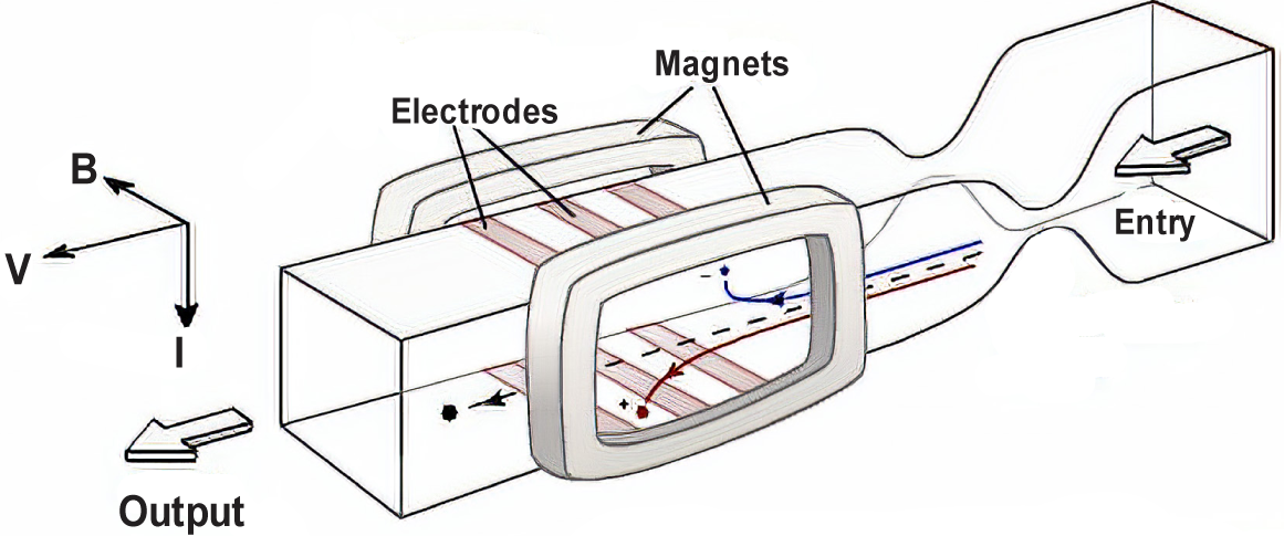
Magnetohydrodynamic generator (MHDG) has been a research topic since the 1890s when Michael Faraday established its fundamental principle [3]. In principle, electric power generation is achieved by an electrically conductive fluid as it flows through a duct subjected to a magnetic field of appropriate strength. One side of the duct walls, compromising electrical electrodes, is perpendicular to both directions of the electrically conductive liquid metal flow and the magnetic field. Electric current is generated and picked by these electrodes. The remaining duct walls are entirely electrically insulated [4]. The schematic of a typical MHDG system is shown in Figure 1.
Schematic of Magnetohydrodynamic power generator [1]
The velocity and electrical conductivity of the working fluid as well as the strength of the magnetic field, have been recognized as key factors in determining the MHDG performance. For a working fluid, there are certain magnetic fluids to choose from; Ionized gases and liquid metal (LM) are the most common. However, ionized gases only achieve the desired electrical conductivity at very high temperatures [5]-[7]. On the other hand, LM has much higher electrical conductivity and works well at considerably lower temperature conditions, resulting in a more reliable MHDG system that can be easier to build and is more suited to work with permanent magnets [8].
According to the number of working fluids, LMMHD systems are divided into single-phase and two-phase systems. In the single-phase system, the electrically conductive liquid is pumped through conduits [9]-[12]. In the two-phase system, the electrically conductive liquid is driven through the magnetic field by gas forced into the system at high velocity, forming a multi-phase flow [13]-[14]. As such, a two-phase system requires a mixing section before admitting into the generator and a downstream separator to retrieve the gas for reuse; this complicates the system and reduces efficiency. To overcome this problem, Lu et al. [8] introduced a self-evaporating driving LMMHD system design, where the liquid metal with a low-boiling point is driven by its own vapor. To generate the vapor, the liquid fluid must be heated to a temperature above its boiling temperature [8]. The supplied heat adds to the overall power input to the MHDG system. The most recognizable advantage of using single self-evaporating fluid is the dispensing with the mixer and separator.
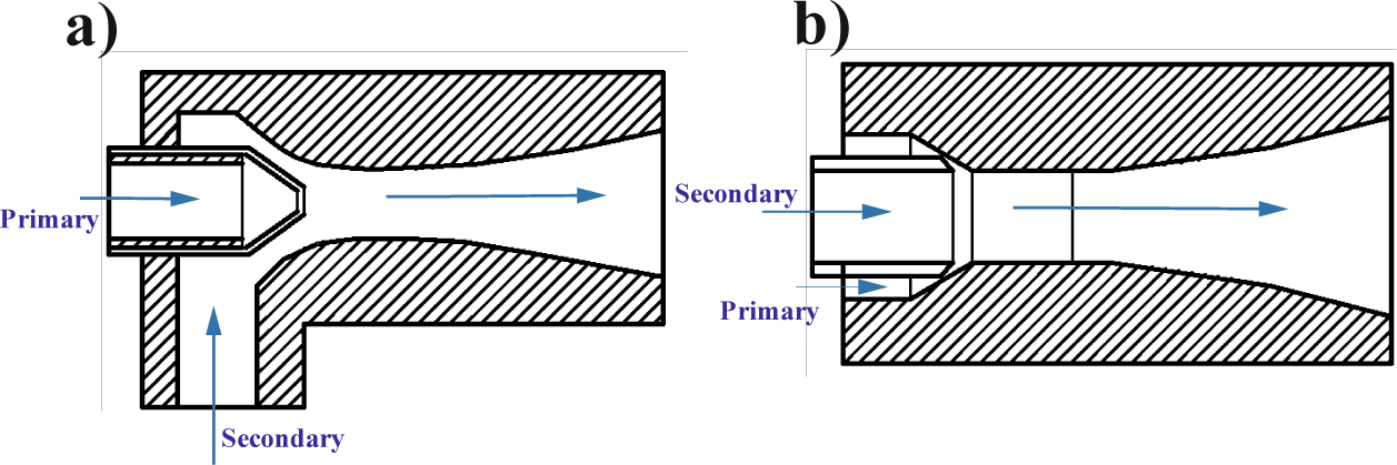
Adding the ejector to the system presented by Lu et al. [8] is expected to enhance both the heating process to generate the driving vapor and increase the pumping effect for the system, thus increasing the generated power. The ejector as a pumping device is commonly utilized in multi-phase flow. And there are two main types of ejectors: axial ejectors and circumferential ejectors. They differ by the nozzle arrangement (Figure 2) through which the forced/ produced gas ejects the liquid. The axial ejectors are the most common; many models have been presented to study the performance of the axial ejector. The simplest is a zero-dimensional model [15], which assumes thermodynamic and mechanical equilibrium over the fluid domain. Such a "lumped" model does not allow a spatial analysis of the key parameters [16]. Liu and Groll [17] proposed a technique for calculating the performance of axial ejectors by formulating empirical correlations to estimate motive nozzle, suction nozzle, and mix section performances. They found that the performance of ejector elements changes with different geometries and conditions. Huang et al. [18] presented an experimentally validated one-dimensional analysis to study the performance of the axial ejector at critical-mod operation assuming constant-pressure mixing and chocked entrained flow.
Types of ejectors: axial ejector (a); circumferential ejector (b) [16]
Many researchers [19]-[23] utilized CFD to conduct multi-dimensional modeling allowing a better tool to investigate and predict the pumping performance of the axial ejector and to account for variations in the ejector geometry and the operating conditions as well to provide a local characterization of the flow throughout the ejector. Wu et al. [19] utilized CFD to simulate a one-dimensional axial ejector model. They carried out a parametric study on two stages for optimization of the ejector: the first one is the single-parameter test which shows how those parameters affect the performance, then the multi-parameters test was performed on many levels. The results reveal that the optimized ejector was the highest performance, and the diameter of the nozzle outlet was the most significant effect parameter on the ejector performance. Colarossi et al. [20] used CFD to simulate a two-dimensional axial ejector model; they found that the boundary conditions at the inlet and the turbulence model are the most sensitively influencing the pressure recovery and accuracy of the ejector model. Also, Yuan et al. [21] used CFD to simulate a three-dimensional axial steam ejector, which calculated velocity and pressure distributions over the fluid domain; they concluded that the entrainment ratio rises dramatically as the inlet pressure rises, then falls once the inlet pressure reaches a certain point.
An annular circumferential ejector requires heating the walls of the ejector to generate the driving vapor, which remains more straightforward and energy efficient than forcing a compressed gas, as is the case with the central axial ejector. Lisowski and Momeni [24] used CFD to simulate the annular ejector model. They investigated three designs to study the effect of the motive nozzle's geometry on the performance of the ejector. The results of their study revealed that a modification of the design enhances the pumping effect by 45%.
Lu et al. [8] introduced a self-evaporating driving LMMHD system design, where the liquid metal is driven by its own vapor. This paper investigates the effect of using a circumferential annular ejector on the performance of a self-evaporating MHD system. The expected result of adding this device is easing the heating process to generate the driving vapor, thus improving the pumping action and increasing the generated power. The performance of this system in terms of velocity augmentation and MHD power density is calculated and presented in terms of vapor/liquid ratio, heat input power, and nozzle ejector configuration.
CFD is a new product that combines computer science and mathematics, and it has proven to be quite successful in simulating ejectors. Moreover, a comparison of various studies shows that CFD errors are more tolerable than conventional 1D or 2D methodologies, despite some disparities between measured and CFD computed outcomes; CFD may be used to reliably anticipate experimental findings, whereas experiments require a lot of time and cost.
This part presents the problem statement, mathematical model, and numerical method.
CFD is used to investigate the performance of a self-evaporating MHD system by utilizing a circumferential ejector. Moreover, liquid sodium is used as the working fluid. The system's performance in terms of velocity augmentation and MHD power density are calculated and presented in terms of vapor/liquid ratio, heat input power, and nozzle ejector configuration. Figure 3 shows the schematics of the proposed system.
The schematic diagram of ejector
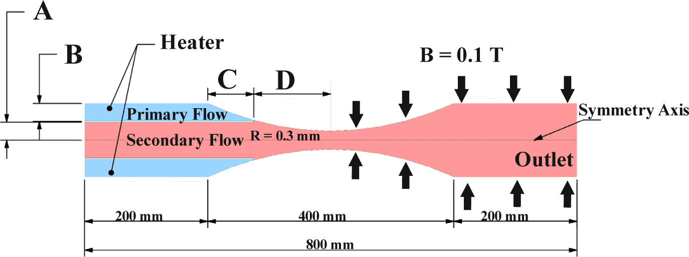
These cases are selected to cover a variety of possible circumferential ejector configurations and to identify the optimal or near-optimal one. Five different cases and four geometrical parameters are taken for the off-design operation. The parameters A, B, C, and D are the radius of the secondary inlet, the difference between the outer radius and inner radius, an axial distance over 200 mm that is added to the primary region, and the distance between the two throats (primary throat and main throat), respectively. In case 1, no distance is added to the primary region (C =0), which means no change in the cross section of the primary region happened. While in case 2, the parameter C is 31 mm, where the smallest diameter of the primary throat is at this value. However, the dimensions of the considered ejector configurations are listed in Table 1.
Parameters of the proposed system
| A | B | C | D | |
|---|---|---|---|---|
| Case 1 | 4.88 | 14.63 | 0 | 200 |
| Case 2 | 4.88 | 14.63 | 31 | 169 |
| Case 3 | 9.75 | 9.75 | 64.63 | 135.37 |
| Case 4 | 9.75 | 9.75 | 75 | 125 |
| Case 5 | 14.63 | 4.88 | 155 | 45 |
Assuming a 2D steady flow mixture of the liquid metal and its vapor, the governing equations can be presented as [25]:
The continuity equation for the mixture is:
(1)
where is the mass-averaged velocity and is the mixture density.
αk is the volume fraction of phase k where n = 2 for this case. Phase 1 is the liquid metal, and phase 2 is its vapor:
(2)
The momentum equation for the mixture is:
(3)
The term on the left-hand side of eq. (3) is the rate of momentum transfer, and the terms on the right-hand side are the pressure force, the viscous stresses, the gravity body force, the Lorentz force, and the drift force between interphases, respectively. j is the current density, B is the magnetic field intensity, μm is the viscosity of the mixture, which is equal to and is the drift velocity for secondary phase k, which is equal to .
The energy equation for the mixture takes the following form:
(4)
The term on the left-hand side of equation (4) is the enthalpy carried by the mixture, and the terms on the right-hand side are the axial conduction, the viscous dissipation, and the energy caused by the Lorentz force, respectively. In this equation, keff is the effective conductivity , Kt is the turbulent thermal conductivity, and E is the electric field.
In addition, the k-ε turbulence model is used in this work. The equations of the turbulence model can be referred to in references [24], [25].
The continuity equation for current is:
(3)
Ohm's law is:
(4)
where σ is the electric conductivity.
The electric field is:
(5)
where φ is the electrical potential which can be calculated by using equation (6):
(6)
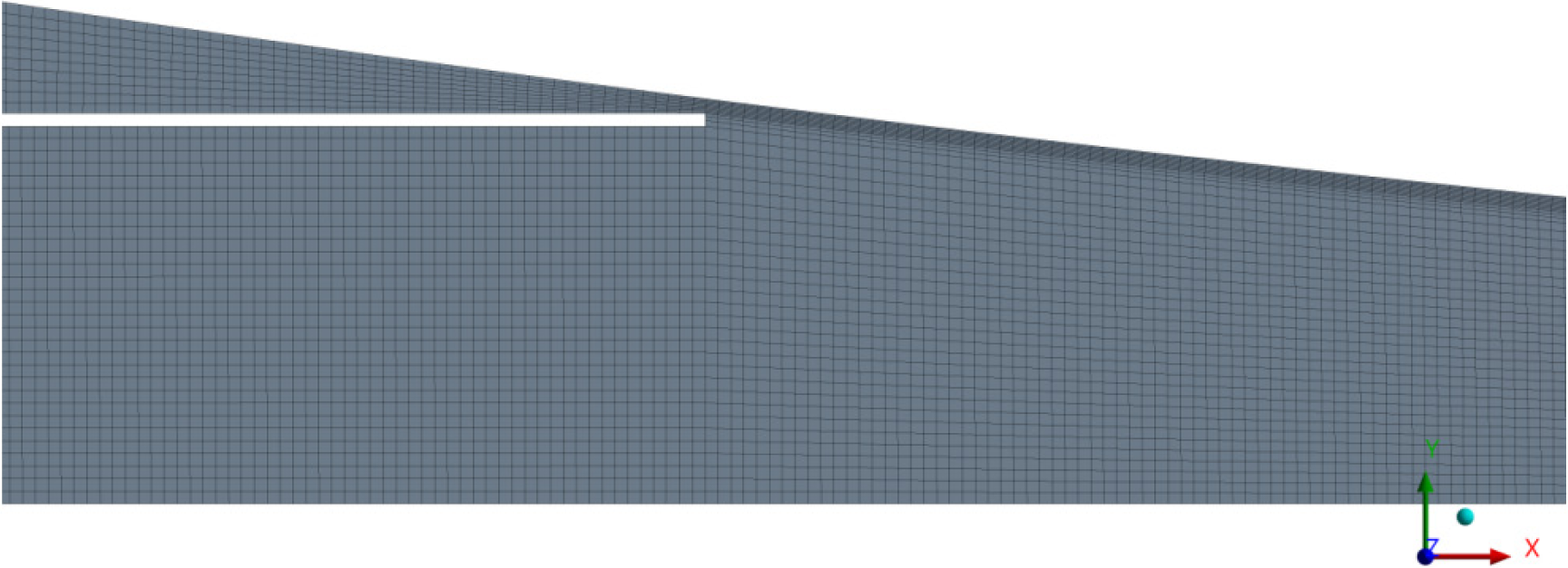
The geometrical modeling and meshing of the five test cases (Table 1) are conducted using ANSYS-FLUENT. To ensure numerical stability, hexahedral mesh grids were structured using the MultiZone Qua/Tri method with face meshing. Mesh generation nearing the primary and secondary nozzle throat is shown in Figure 4.
Mesh structure near the nozzle throat
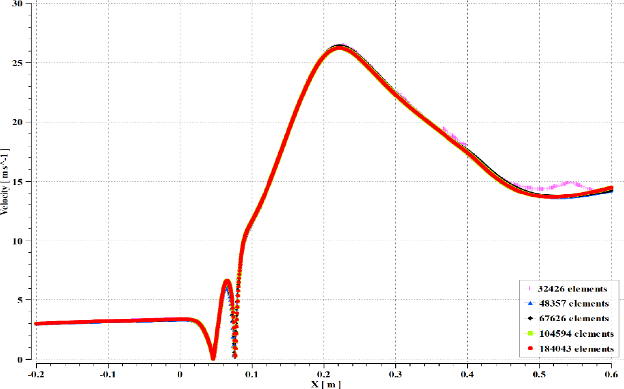
Grid sensitivity analysis is conducted by using the incrementally refined mesh sizes of 32426, 48357, 67626, 104594, and 184043. Figure 5 shows the velocity distribution of liquid sodium along the central x-axis. The difference between the course and the finer mesh size is lower than 1.1%. Therefore, mesh sizes 48357 and 67626 elements were applied throughout the present study.
Velocity distribution of liquid sodium along the central x-axis at different element size
The governing equations are solved numerically by using the finite volume method by ANSYS-FLUENT. The Mixture and MHD models [25], [28] are utilized for simulating the multi-phase flow under a magnetic field. The Evaporation-Condensation model is embedded to solve the interaction between the phases [25]. SIMPLE scheme is used for the pressure-velocity coupling. The least-square cell-based method is used for computing the cell-centered spatial gradient terms and the second-order discretization scheme for the convective terms in the pressure and density equations. The volume fraction is discretized using QUICK scheme. Table 2 shows the physical properties of liquid Sodium and its vapor at Tref. =1155 K [8]. Density, thermal conductivity, electrical conductivity, latent heat of vaporization, magnetic permeability, and viscosity are all assumed constant. The k-ε two-equation turbulent model with standard wall functions is employed. Symmetry boundary conditions are applied along the centerline of the ejector.
Physical properties of liquid sodium and its vapor
| Physical properties | liquid sodium | sodium vapor |
|---|---|---|
| Molar mass (g·mol-1) | 22.9 | 22.9 |
| Density (kg·m-3) | 927 | 1.7 |
| Boiling point (K) | 1156 | - |
| Heat capacity (J·kg-1·K-1 | 1281.9 | 1300.0 |
| Latent heat of vaporization (kJ·kg-1) | 3521.5 | - |
| Thermal conductivity (W·m-1·K-1) | 50.0 | 59.2 |
| Viscosity (kg·m-1·s-1) | 0.2 * 10-3 | 3.3 * 10-6 |
| Electrical conductivity (siemens /m) | 2 * 107 | 100 |
| Magnetic permeability | 1.2 * 10-6 | 1.2 * 10-6 |
The validation and all results are presented in this part.
To validate the new model, Lu et al. [8] geometry is modeled with the same dimensions that they used. Grid sensitivity analysis is conducted by using the incrementally refined five mesh sizes, as shown in Figure 5. The governing equations are solved numerically using the methods presented in the previous section. The outlet boundary condition was pressure-outlet with atmospheric conditions, whereas the inlet boundary condition was velocity-inlet. Despite the strong coupling between the equations introduced in mathematical model section, convergence is achieved with precision 10-6 of the residual monitor. The solution procedure is described in the following:
Solve for the multi-phase flow, MHD deactivated. With the solution of multi-phase flow converged, activate the MHD model. Repeat the previous two steps until full convergence is achieved. In some cases, it may be needed to lower under-relaxation factors.
Lu et al. [8] case (without the circumferential annular ejector) is resolved using the above methodology. As shown in Figure 6, Figure 7 and Figure 8, our findings coincide very closely with Lu et al. [8]. The discrepancy ranged 0.027-0.75% for the outlet velocity, 0.29 -3.96% for the liquid outlet volume fraction, and 0.52 - 1.13% for the outlet temperature under the same conditions. We used Lu et al. [8] test cases as reference cases. They simulated a conventional Self-Evaporating LMMHD system, which did not contain the ejector device. Contrary to their system, we added a circumferential ejector to investigate the effect of adding this device on the system's performance where the one entrance they used divide to two entrances, primary and secondary.
Figure 6 shows the effect of wall temperature on the outlet velocity. Regardless of whether an ejector is used or not, it is evident that increasing the wall temperature increases the outlet velocity. At 1337 K, the outlet velocity is 7.44 m/s for case 1 and 9.09 m/s for case 2. The higher the wall temperature, the higher the outlet velocity; so, using the ejector increases the outlet velocity in most cases except case 1, where no change in the cross section of the primary region happened. Case 2 shows the most effective case, where the outlet velocity is increased by 18.36% due to the ejector compared with the case without the ejector at 1773K.
The effect of wall temperature on the outlet velocity with and without ejector
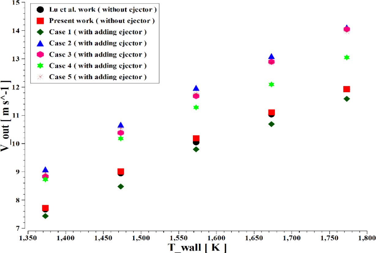
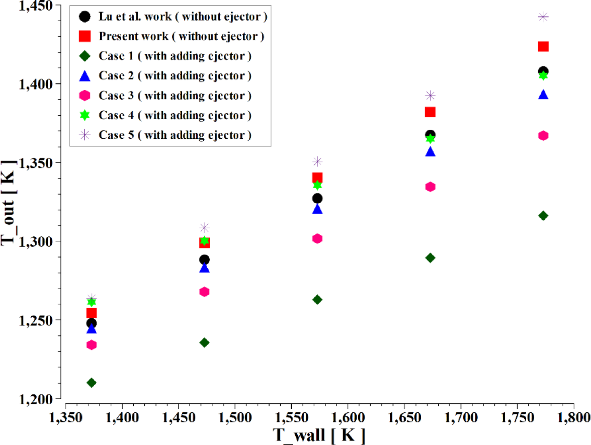
Figure 7 shows that increasing the wall temperature increases the outlet temperature in all cases. At 1337 K, the outlet temperature is 1263.6 K for case 5 and 1210.2 K for case 1. The outlet temperature gradually increases as the wall temperature increases to 1773K. Using the annular ejector with different parameters affects the outlet temperature; contrary to cases 1,2 and 3, the outlet temperature in case 5 increases by 2.46% while it decreases by 6.51% in case 1.
The effect of wall temperature on the outlet temperature with and without ejector
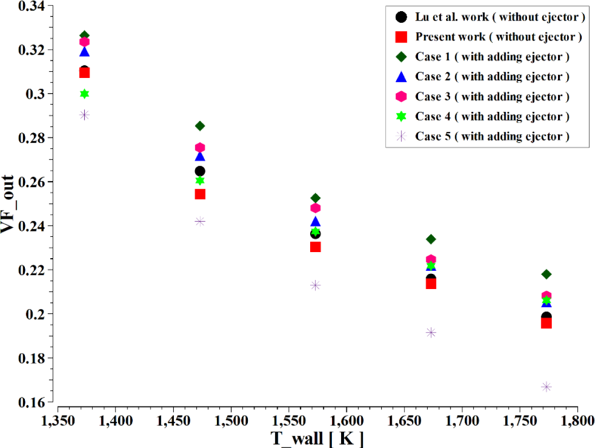
The wall temperature increases leading to sodium LM evaporation. Figure 8 shows that increasing the wall temperature reduces the outlet volume fraction of liquid in all cases. The outlet volume fraction of liquid at 1337 K wall temperature is 0.376 for case 1 and 0.29 for case 5. The outlet volume fraction of liquid declines steadily as the wall temperature. Figure 8 also shows that the annular ejector affects the outlet volume fraction of liquid which increases by 21.24% in case 1 and decreases by 16% in case 5 compared with the reference case at 1773K wall temperature when the ejector was not used. Temperature increases, reaching 0.25 for case 1 and 0.17 for case 5 at 1773K wall.
The effect of wall temperature on the outlet volume fraction of liquid with and without ejector
As the previous section demonstrates, increasing the wall temperature can result in a higher outlet velocity, which is beneficial to output power but also results in a lower volume fraction of liquid. Reduced liquid volume fraction (more vapor phase) accelerates the mixture but reduces its electrical conductivity.
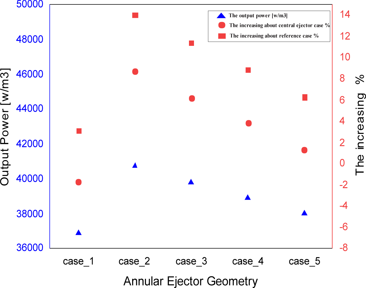
The output power was computed for all cases in this section using a constant magnetic field of 0.1 T. All five proposed geometries for the annular ejector and geometry for the central ejector is compared with the reference case (without ejector). The findings show that the output power has increased in all cases when using the ejector. Figure 9 and Table 3. show that the increase of output power due to increased velocity is higher than the loss in power due to the decrease in the volume fraction of the liquid.
The effect of ejector geometry on the output power
| Ejector geometry | J [a/m2] | E [V/m] | P [W/m3] | The increasing % |
|---|---|---|---|---|
| Ref. case | 30360.8 | 1.8 | 35753.1 | - |
| central ejector | 37071.0 | 1.0 | 37495.6 | 4.9 |
| case_1 | 35930.9 | 1.0 | 36870.7 | 3.1 |
| case_2 | 35400.4 | 1.2 | 40771.5 | 14.0 |
| case_3 | 35134.0 | 1.1 | 39828.3 | 11.4 |
| case_4 | 34170.3 | 1.1 | 38930.5 | 8.9 |
| case_5 | 39755.3 | 1.0 | 38007.5 | 6.3 |
As shown in Figure 9, case 2 is the best geometry that gives the maximum output power augmentation. For case 2, output power increases by 14.0% over the reference case (without ejector) and 8.7% over the central ejector case.
The effect of the annular ejector on the output power
In the next section, the analysis will focus on the performance of the best case, case number 2, where the velocity, temperature, pressure, and volume fraction distributions are presented.
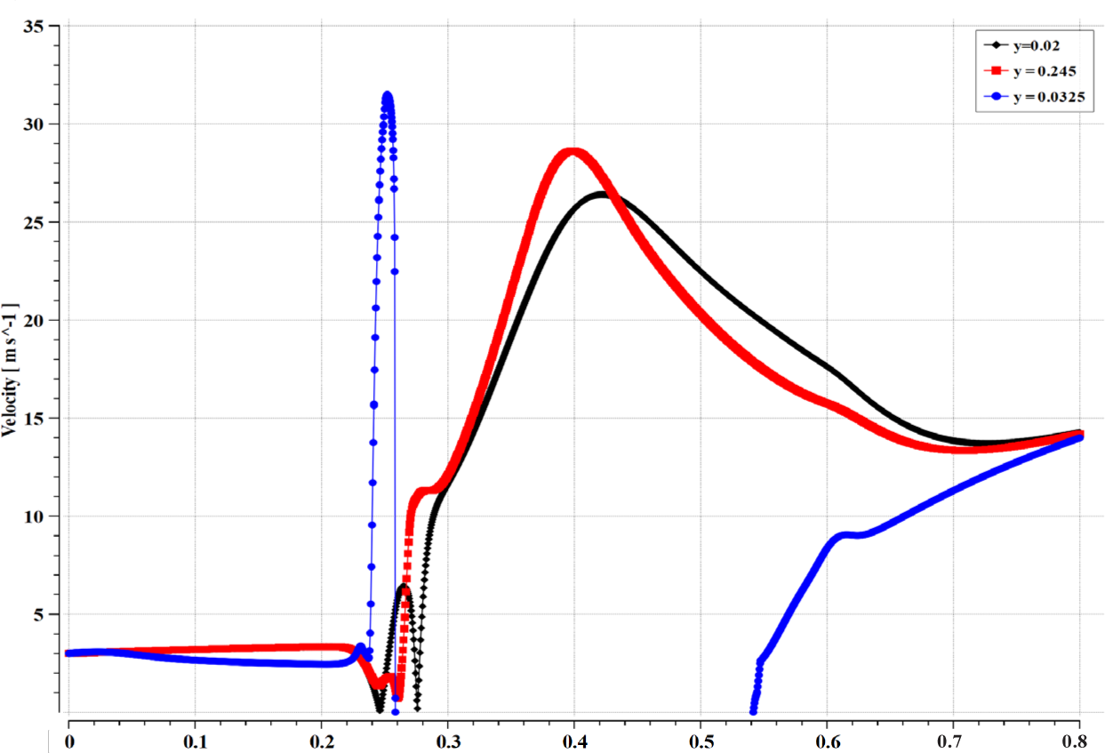
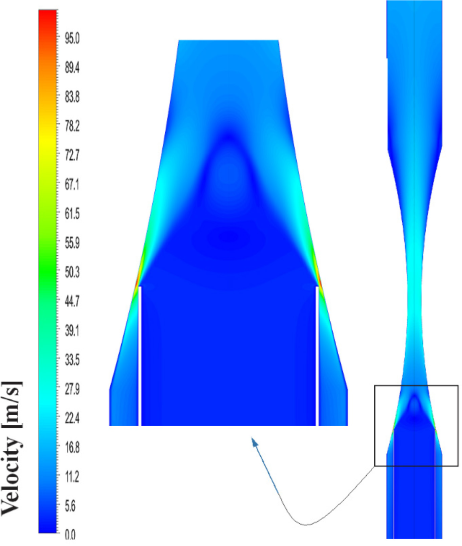
Figure 10, Figure 11, and Figure 12 present the contours of velocity in an annular ejector, the velocity distribution along the x-axis, and the velocity distribution along the y-axis. As shown in these figures, the sodium LM is admitted at a velocity of 3 m/s for primary and secondary nozzles. In the primary nozzle, part of the sodium LM starts converting to vapors which causes acceleration in the primary flow to reach around 90 m/s at the throat of the ejector. Then the velocity decreases due to the momentum exchange between the primary and the secondary flows. The velocity of the primary flow continues to drop to reach the same value as the secondary flow through the diffuser. Finally, bubbly flow leaves the MHD channel with a velocity of around 15 m/s.
Distribution of velocity [m/s] along X at different Y position
The contour of velocity [m/s] for case 2
Distribution of velocity [m/s] along Y at different X position: at X= 0.1, 0.2 0.264 and 0.3(a); at X= 0.4, 0.5, 0.6 and 0.7 (b)
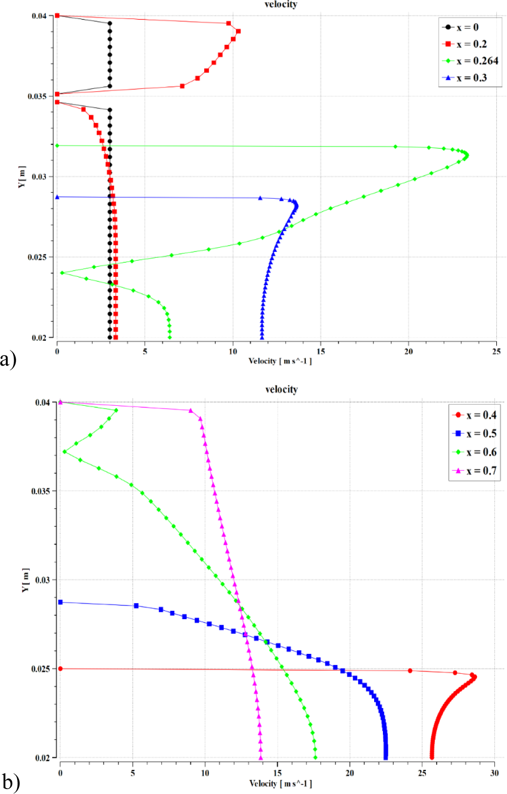
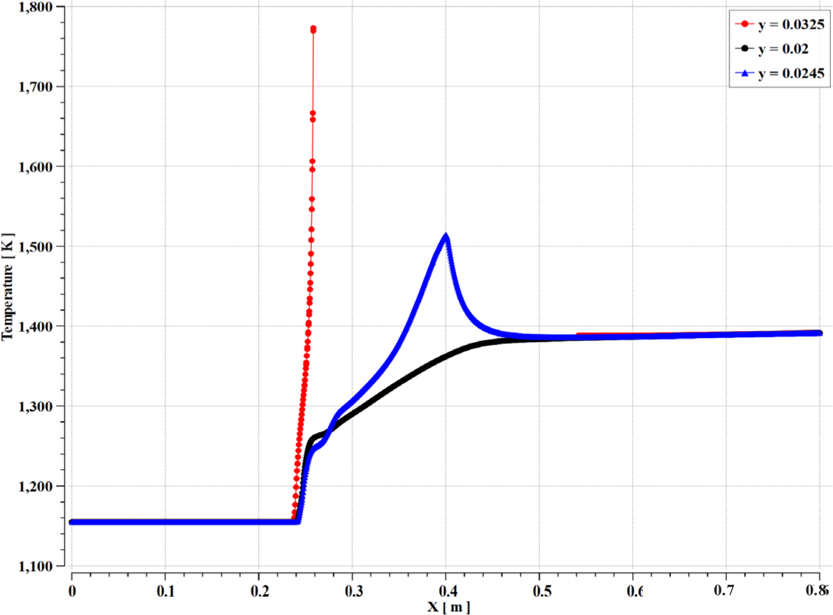
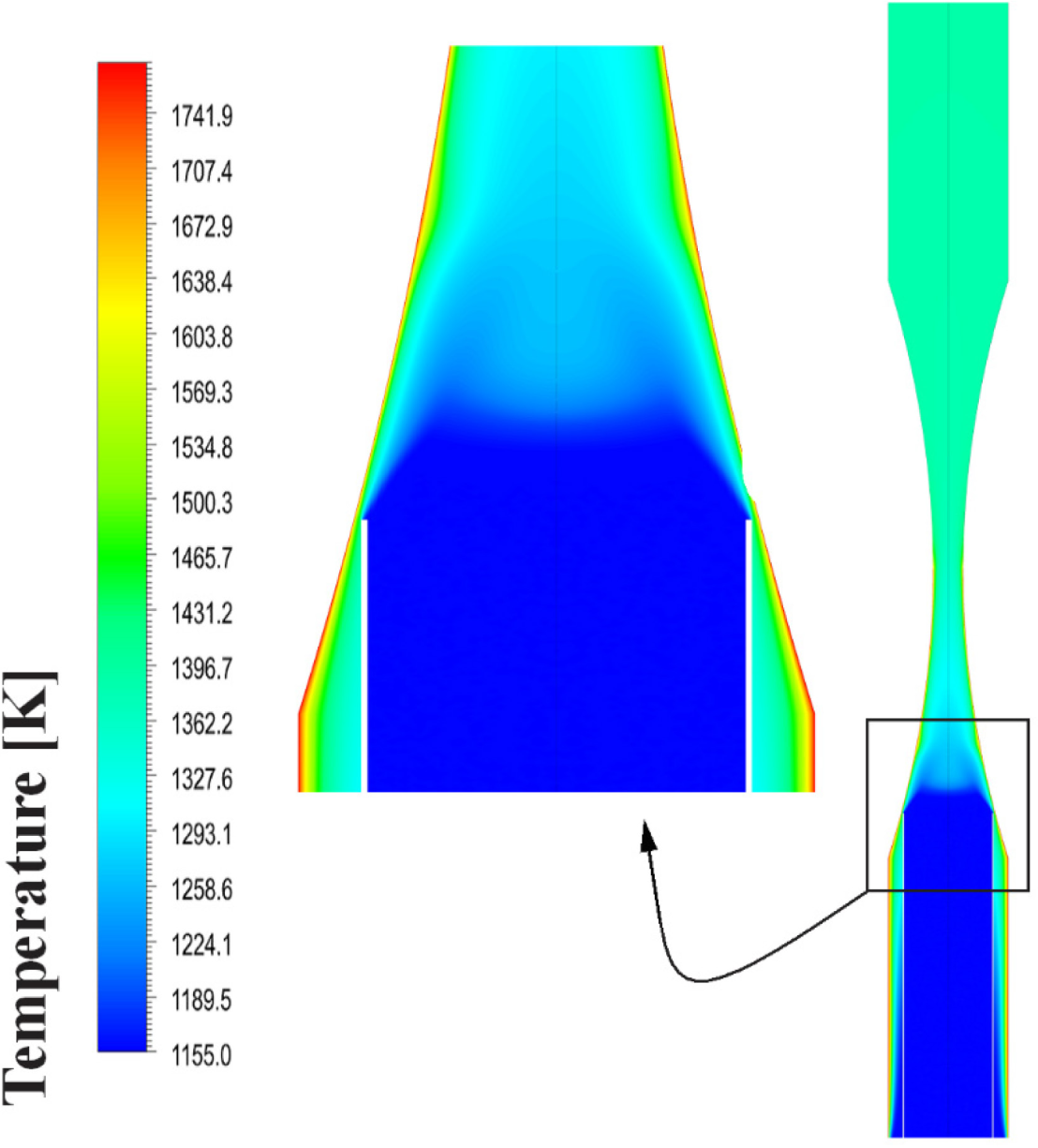
Figure 13, Figure 14 and Figure 15 present the contours of temperature in the annular ejector, the temperature distribution along the x-axis, and the temperature distribution along the y-axis. As shown in these figures, the sodium LM enters with a temperature of 1155 K, less than the sodium's boiling point by 1 K. The heat transfer occurs from the heated wall to the primary at a flux of 7.4×10⁵ W, which causes evaporation of the liquid metal in the annular ejector. At the throat, two stream mix together. The temperature of the primary flow continues dropping to reach the same value as the secondary flow through the diffuser. Finally, the mixture leaves the MHD channel at a temperature of around 1400 K.
Distribution of temperature [K] along X at different Y position
The contour of temperature [K] for case 2
Distribution of temperature [K] along Y at different X position: at X= 0.1, 0.2 0.264 and 0.3 (a); at X= 0.4, 0.5, 0.6 and 0.7 (b)
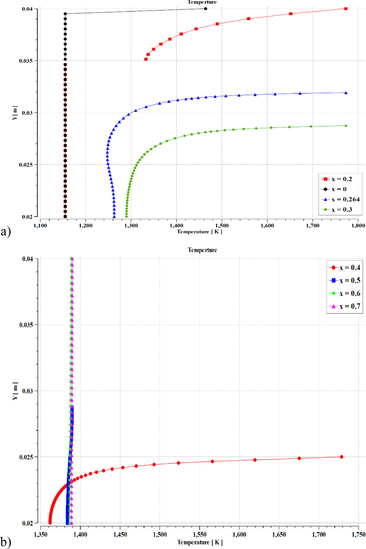
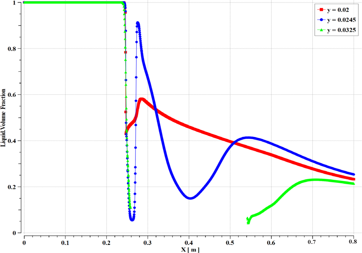
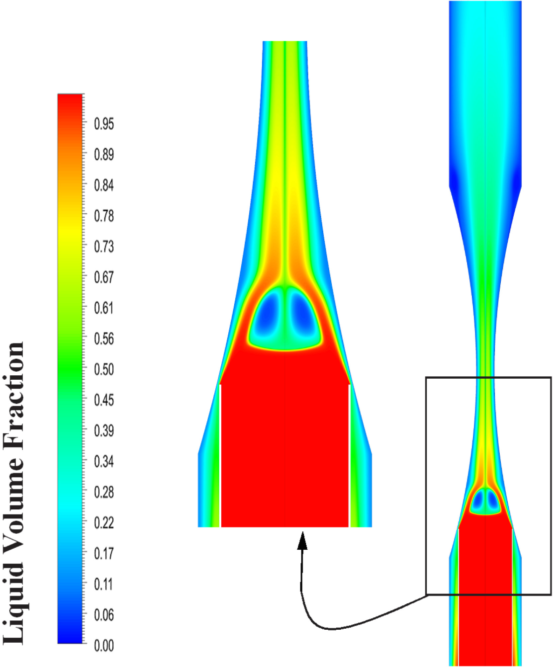
Figure 16, Figure 17 and Figure 18 present the volume fraction contours of liquid in an annular ejector, the volume fraction of liquid distribution along the X-axis, and the volume fraction of liquid distribution along the Y-axis. These figures show that; the volume fraction of liquid is dominant at the beginning; then part of the primary stream converts to sodium vapor due to heating, while the secondary one remains liquid until two streams mix after the throat. Bubbly flow occurs in the diffuser and leaves the MHD channel with a volume fraction of liquid around 22%.
Distribution of liquid volume fraction along X at different Y position
The contour of liquid volume fraction for case 2
Distribution of liquid volume fraction along Y at different X position: at X= 0.1, 0.2 0.264 and 0.3 (a); at X= 0.4, 0.5, 0.6 and 0.7 (b)
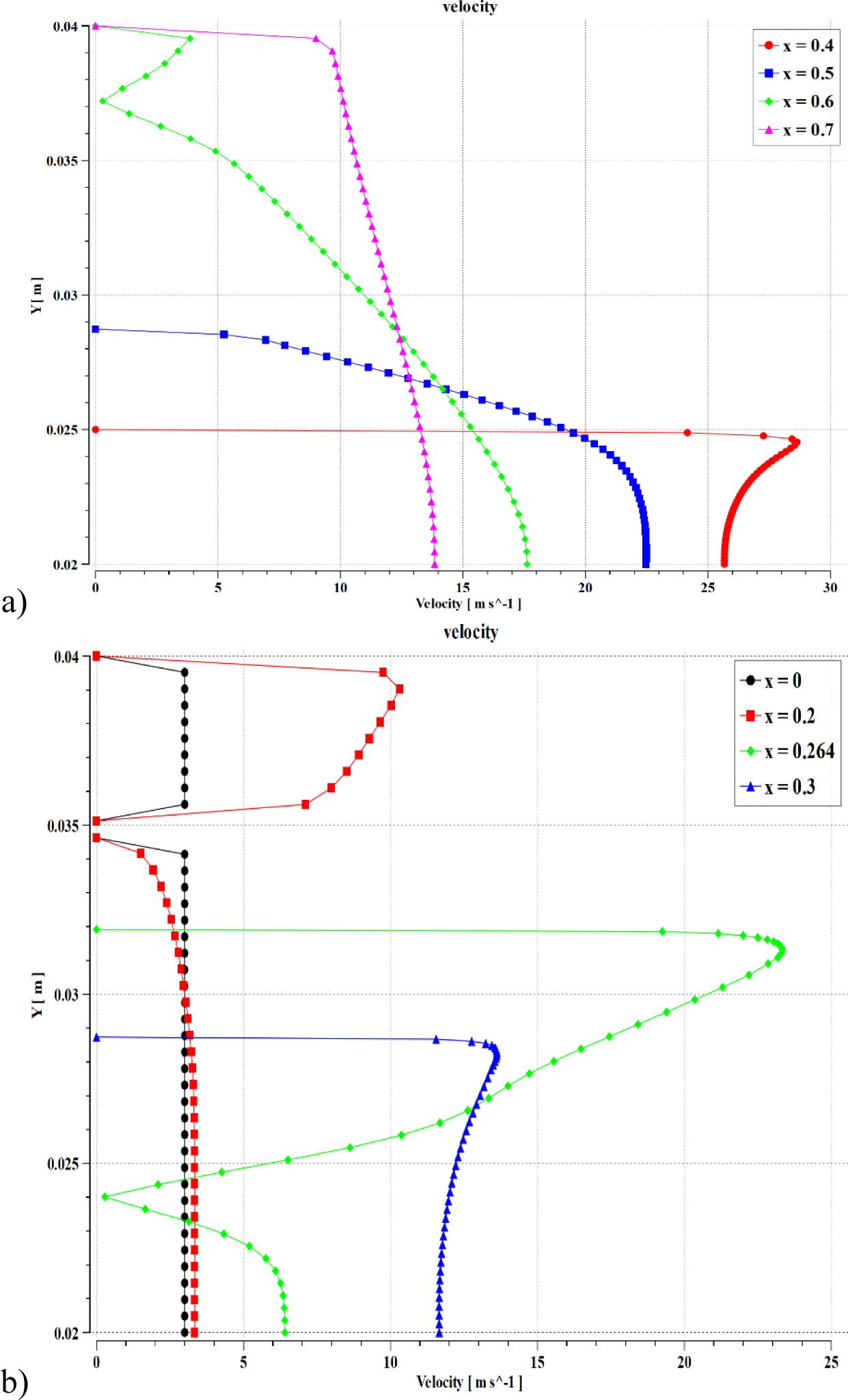
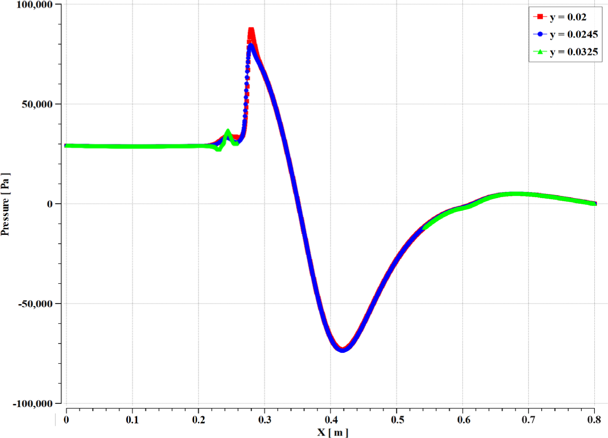
Figure 19 and Figure 20 display the contours of pressure in the annular ejector and the pressure distribution on the X-axis. As demonstrated, the pressure of the primary stream as it passes through the primary region drops dramatically and then falls to a lower value near the main throat, where vacuum and momentum transfer between the two streams occur in the mixing region after the throat. Driven by the pressure gradient, the secondary stream accelerates by the primary stream. Finally, the mixture leaves the MHD channel with atmospheric pressure imposed as a boundary condition.
Distribution of pressure [Pa] along X at different Y position
The contour of pressure [Pa] for case 2

The entrainment ratio is the ratio of the primary stream's mass flow rate to the secondary stream's mass flow rate. It measures the amount of the secondary fluid driven by the primary one. The effect of the entrainment ratio on power density was investigated using a magnetic field of 0.1 T, a wall temperature of 1773K, a density of sodium liquid metal of 927 kg/m3, an area of primary section is 7.5×10⁻⁵ m2, and the area of the secondary section is 6.7×10⁻⁴ m2.
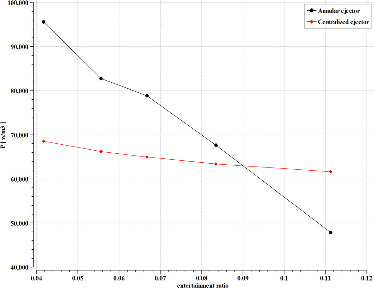
Figure 21 and Table 4 show that raising the entrainment ratio reduces the power density. This power reduction is characterized by a decline in the mass flow rate of the secondary stream, i.e., the flow through the generator becomes more diluted, thus less power generation. At the entrainment ratio of 0.04172, the power density is 95.613 kW/m3 for the annular ejector and 68.558 KW/m3 for the central ejector. It decreases gradually as the entrainment ratio increases; at a 0.1113 ratio, the generated power becomes 47.853 kW/m3 for the annular ejector and 61.629 KW/m3 for the central ejector.
The effect of entrainment ratio on power density
The effect of entrainment ratio on power density
| Entrainment ratio | P [W/m3] (annular ejector) | P [W/m3] (central ejector) |
|---|---|---|
| 0.042 | 95613.2 | 68557.9 |
| 0.056 | 82775.4 | 66202.5 |
| 0.067 | 78856.3 | 64968.3 |
| 0.083 | 67654.3 | 63399.2 |
| 0.111 | 47852.8 | 61628.8 |
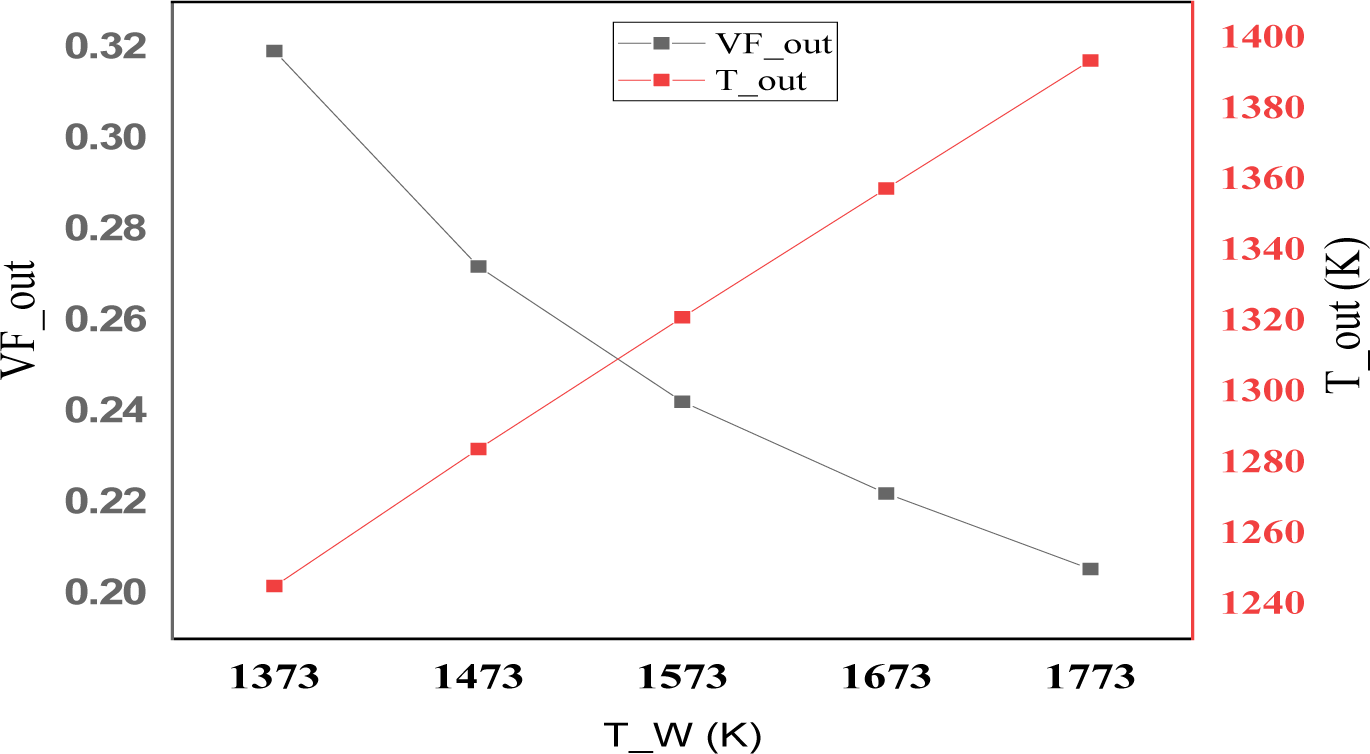
With the increased input heating power and, therefore, the increased wall temperature, more vapor phase is generated to drive the mixture. Speeding up the mixture counterweighted the adverse effect of reducing the volume fraction of the electrically conductive liquid and resulted in a higher net power generation. Figure 22 shows the optimum value of the heat added that delivers the maximum performance in case 2.
The effect of wall temperature on the outlet parameters, case 2
CFD was used in this study to simulate a two-dimensional single-loop LMMHD system driven by a circumferential annular ejector. Sodium LM is used as the working fluid. The Mixture model and the MHD model are utilized to simulate the multi-phase flow through a magnetic field. The Evaporation-Condensation model is embedded to describe the interaction between the two phases, the liquid metal and its vapor.
The parametric analysis and optimization involved the geometry of the annular ejector, input heating power, and the entrainment ratio. More detailed analyses were carried out for the optimal case, where power density assumes maximum value. Velocity, pressure, temperature, and liquid and vapor fraction distributions are presented and analyzed. Adding a circumferential annular ejector to the self-evaporating driving LMMHD device proved feasible.
Pumping more flow rate means higher liquid metal velocity, thus larger power density. Adding a circumferential annular ejector boosted the velocity of the working fluid by 18% in comparison with the system without an ejector and by 12.9% compared to the system with a central axial ejector when considering the optimum case 2. Thus, incorporating a circumferential annular ejector into the system contributed to improvement in the system performance.
Further work based on economic studies and energy analysis should be carried out, especially when using this technique in a combined cycle.
- ,
The Future Power Generation with MHD Generators Magneto Hydro Dynamic generation ,Int. J. Adv. Electr. Electron. Eng. , Vol. 2 (6), 2013 - ,
Open-cycle magnetohydrodynamic electrical power generation: A review and future perspectives ,Prog. Energy Combust. Sci. , Vol. 30 (1),pp 33-60 , 2004, https://doi.org/https://doi.org/10.1016/j.pecs.2003.08.003 - ,
History of MHD power plant development ,Energy Convers. Manag. , Vol. 37 (5),pp 569-590 , 1996, https://doi.org/https://doi.org/10.1016/0196-8904(95)00212-X - ,
The Magnetohydrodynamic Power Generator: Basic Principles, State of the Art, and Areas of Application ,IRE Trans. Mil. Electron. , Vol. 6 (1),pp 78-83 , 1962, https://doi.org/https://doi.org/10.1109/IRET-MIL.1962.5008403 - ,
Numerical simulation of power generation characteristics of a disk MHD generator with high-temperature inert gas plasma ,Electr. Eng. Japan , Vol. 179 (3),pp 23-30 , 2016, https://doi.org/https://doi.org/10.1002/eej.21237 - ,
Plasma characteristics and performance of magnetohydrodynamic generator with high-temperature inert gas plasma ,IEEE Trans. Plasma Sci. , Vol. 42 (12),pp 4020-4025 , 2014, https://doi.org/https://doi.org/10.1109/TPS.2014.2365591 - ,
Experiments on High-Temperature Inert Gas Plasma MHD Electrical Power Generation with Hall and Diagonal Connections ,Electr. Eng. Japan , Vol. 193 (3),pp 17-23 , 2015, https://doi.org/https://doi.org/10.1002/eej.22761 - ,
Numerical Investigation on the Characteristics of Vapor-liquid Flow in the Heater of Self-evaporating- driving Liquid Metal Magneto-hydro-dynamic System ,Ind. Eng. Chem. Res. , Vol. 56 (35),pp 9917-9925 , 2017, https://doi.org/https://doi.org/10.1021/acs.iecr.7b02550 - ,
Numerical simulation of MHD effects on convective heat transfer characteristics of flow of liquid metal in annular tube ,Fusion Eng. Des. , Vol. 86 (2-3),pp 183-191 , 2011, https://doi.org/https://doi.org/10.1016/j.fusengdes.2010.11.009 - ,
Numerical investigation of a thermosyphon MHD electrical power generator ,Energy Convers. Manag. , Vol. 187 ,pp 378-397 , 2019, https://doi.org/https://doi.org/10.1016/j.enconman.2019.02.085 - ,
Numerical examination of liquid metal magnetohydrodynamic flow in multiple channels in the plane perpendicular to the magnetic field ,J. Mech. Sci. Technol. , Vol. 28 (12),pp 4959-4968 , 2014, https://doi.org/https://doi.org/10.1007/s12206-014-1117-z - ,
Numerical simulation of 3D magnetohydrodynamic liquid metal flow in a spatially varying solenoidal magnetic field ,Fusion Eng. Des. , Vol. 156 , 2020, https://doi.org/https://doi.org/10.1016/j.fusengdes.2020.111659 - ,
Feasibility analysis of two-phase MHD energy conversion for liquid metal cooled reactors ,Nucl. Eng. Des. , Vol. 237 (20-21),pp 2114-2119 , 2007, https://doi.org/https://doi.org/10.1016/j.nucengdes.2007.02.009 - ,
, Numerical investigation into the vapor-liquid flow in the mixer of a liquid metal Magneto-Hydro-Dynamic system , - ,
, Vol. 7 (57), pp 35765-35770 , 2017, https://doi.org/https://doi.org/10.1039/C7RA06135H - ,
The use of an ejector in a geothermal flash system ,Proc. Intersoc. Energy Convers. Eng. Conf. , Vol. 5 ,pp 79-84 , 1990 - ,
Transcritical CO2 refrigeration cycle with ejector-expansion device ,Int. J. Refrig. , Vol. 28 (5),pp 766-773 , 2005, https://doi.org/https://doi.org/10.1016/j.ijrefrig.2004.10.008 - ,
Study of ejector efficiencies in refrigeration cycles ,Appl. Therm. Eng. , Vol. 52 (2),pp 360-370 , 2013, https://doi.org/https://doi.org/10.1016/j.applthermaleng.2012.12.001 - ,
A 1-D analysis of ejector performance Analyse unidimensionnelle de la performance d ' un e , Vol. 22 ,pp 354-364 , 1999, https://doi.org/https://doi.org/10.1016/S0140-7007(99)00004-3, November 1998 - ,
Optimization analysis of structure parameters of steam ejector based on CFD and orthogonal test ,Energy , Vol. 151 ,pp 79-93 , 2018, https://doi.org/https://doi.org/10.1016/j.energy.2018.03.041 - ,
Multidimensional modeling of condensing two-phase ejector flow ,Int. J. Refrig. , Vol. 35 (2),pp 290-299 , 2012, https://doi.org/https://doi.org/10.1016/j.ijrefrig.2011.08.013 - ,
Three-dimensional CFD modeling and simulation on the performance of steam ejector heat pump for dryer section of the paper machine ,Vacuum , Vol. 122 ,pp 168-178 , 2015, https://doi.org/https://doi.org/10.1016/j.vacuum.2015.09.016 - ,
Numerical modeling of two-phase supersonic ejectors for work-recovery applications ,Int. J. Heat Mass Transf. , Vol. 55 (21-22),pp 5744-5753 , 2012, https://doi.org/https://doi.org/10.1016/j.ijheatmasstransfer.2012.05.071 - ,
CFD analysis of a supersonic air ejector. Part I: Experimental validation of single-phase and two-phase operation ,Appl. Therm. Eng. , Vol. 29 (8-9),pp 1523-1531 , 2009, https://doi.org/https://doi.org/10.1016/j.applthermaleng.2008.07.003 - ,
CFD modelling of a jet pump with circumferential nozzles for large flow rates ,Arch. foundry Eng. , Vol. 10 (3),pp 69-72 , 2010 - ,
ANSYS Fluent Theory Guide , 2013 - , , Lectures in mathematical models of turbulence, 1972
- ,
Numerical Research on the Flow Fields in the Power Generation Channel of a Liquid Metal Magnetohydrodynamic System , Vol. 5 (48),pp 31164-31170 , 2020, https://doi.org/https://doi.org/10.1021/acsomega.0c04379 - ,
Magnetohydrodynamics (MHD) Module Manual ,ISIJ Int. , Vol. 48 (5),pp 584-591 , 2008, https://doi.org/https://doi.org/10.2355/isijinternational.48.584