


Climate change and the recent energy crisis have pointed out the urgent need to move towards fully renewable energy systems [1]. District Heating and Cooling Networks are included among the key technologies for the achievement of this challenging goal [2]. More specifically, if coupled with power-to-heat technologies like air-to-water or water-to-water heat pumps (HP), they could help managing the unpredictable electricity production from renewable energy sources (RES) [3], which makes the operation of the distribution electric grid very complex [4]. In addition, they could allow for the sharing of heat produced from distributed thermal RES [5] and the exploitation of low-temperature waste heat (WH) from industries [6] and data centers [7]. Due to these capabilities, energy planning tools like EnergyPlan [8] or EnergyPro [9] include these systems among the key technologies in the development of 100% renewable energy systems.
District Heating Networks (DHN) are not new technologies, but great advances have been achieved during the last decades, in terms of thermal insulation, reduction of pressure drop, and operating temperature. Regarding the latter, DHNs are typically supplied by centralized combined heating and power plants (CHP) where fossil fuels or biomass are burnt, and they are operated at 85 °C (typical value for 3rd generation DHN) [10]. However, this operating temperature of the networks does not allow for the inclusion of heat from RES or low-temperature WH flows. To solve this problem, the concept of 4th [11] and 5th-generation DHNs has been developed [12]. In the 4th generation, DHNs are operated at a maximum temperature of about 60 °C. In the 5th DH system, the grid is operated at almost ambient temperature with local boosting at the end-user by using heat pumps to achieve the required temperature level [13].
Attention has also been paid to the development of District Cooling Networks (DCN). In this respect, Østergaard et al. [14] provided a clear picture of the time evolution of this technology, by identifying four generations like in DHNs. Interestingly, in 4th-generation DCNs, the cold demand of the users is met not only by diversified cold sources such as centralized systems (e.g., absorption chillers, compression chillers) and natural cooling sources (lakes, excess cold streams) but also with cold sharing among prosumers and consumers, with HPs operated in combined heating and cooling mode and with the implementation of distributed cold storages (such as water tank or seasonal storage).
Considering the recognized role played by DHNs in future energy systems, large efforts have been devoted by researchers to optimize DHN design [15]. Some researchers focused on the need to redesign substations in case of the lower operating temperature of 4th and 5th DHNs [16]. Some authors focused on the benefits achievable by prosumers in DHNs in terms of achievable energy saving and/or the reduction of carbon dioxide emissions [17]. Other studies, instead, focused on cost evaluation in DHNs. For instance, Gudmundsson et al. [18] found that 4th DHNs could lead to greater economic benefits compared to 5th DHNs. Li et al. [19] developed a dynamic price model for DHNs while comparing some criteria to allocate the costs burdening the heat production (e.g., fuels, maintenance, etc.). Tian et al. [20] found that a 5–9% reduction in heat unit cost could be achieved by using solar collectors. Millar et al. [21] found that a 5th DHN allowed for a strong reduction in heat cost. Verda et al. [22] and Catrini et al. [23] showed the potential of Exergoeconomics for allocating capital and operating costs in DHNs. Finally, other authors addressed the issue of proper maintenance schedules in substations to reduce energy consumption [24]. Indeed, the diagnosis of anomalies in heat exchangers of DHN substations is an essential point to assure high comfort levels in buildings, as well as to save energy. Gadd et Werner [25] identified unsuitable heat load patterns, low average annual temperature difference, and poor substation control, as common faults in European DHNs. Kim et al. [26] developed virtual sensors for detecting fouling in DHN substations using datasets measured from a conventional building automation system. Results showed that by using virtual sensors a 61% improvement in the accuracy of fault detection was achieved.
Considering the strong interest in DHNs, it is useful to provide researchers in this field with simple indicators that could provide insights on the following aspects: (i) the rational uses of thermal energy resources with a different thermodynamic “quality” for DHN supply (e.g., WH at different temperatures or thermal energy from CHP plants), (ii) the effects of thermodynamic inefficiencies occurring in heat production and distribution on the cost of the heat supplied to the users, and (iii) the effect of the off-design operation of poorly-maintained substations. The first point is of utmost importance considering that sustainability issues are pushing society to a keen use of limited energy sources. Meantime, as the number of producers will increase (e.g., the presence of prosumers), there is a need to have indicators that classify them not only for the quantity of thermal energy supplied but also for the thermodynamic quality of the heat flows. Only a few papers have addressed the topic of thermodynamic efficiency in DHNs. For instance, Pass et al. [27] carried out an exergy analysis for a bidirectional network, which adopted a single circuit for both heating and cooling. The authors compared exergy destruction in the case of high- and low head load density vs. individual heating and cooling systems, and the effect of pumping on the exergy destruction was also quantified. Dorotić et al. [28] performed an economic, environmental, and exergetic multi-objective optimization of district heating systems. The minimization of exergy destruction led to the phase-out of natural gas-based technologies.
In a previous paper [23], the authors of this work have developed an exergoeconomic modeling of a ring-shaped network for allocating capital and operating costs in DHN systems. The results highlighted the capability of the method in allocating sustained costs among different users, reflecting the effect of irreversibility on the variation of the unit cost of supplied heat. However, the following aspects were not addressed: (i) the capability of the method to account for different quality of heat sources (especially WH), (ii) the effect of the operating temperature of the grid, (iii) the percentage incidence of irreversibility sources in the heat unit cost (iv), the effect of proper design and maintenance of the DHNs substation on the unit cost of heat. To address the previous points, this paper proposes the Exergy Cost Theory (ECT) [29]. More specifically, ECT provides the unit exergetic cost of a given product (e.g., an energy flow or a stream of matter) which quantifies the resources (measured in exergy) used to produce a unit of exergy of the given product. If inefficient processes are involved along the productive chain of a given product, a large irreversibility is generated, and a high exergy cost is consequent. This property has been proven to make it suitable for allocating sustained costs[30], the consumed natural resources [31], and emissions [32] in multi-output systems. Moreover, it could support the diagnosis of malfunction [33] or be assumed as an index for the evaluation of urban sustainability [34].
In the case of DHNs, by using the unit exergetic cost of the heat supplied to the buildings, it is possible to account separately for inefficiencies occurring in the production units (e.g., CHP plant, RES systems, WH recovery, etc.), along the network (e.g., heat losses and pressure drop), and in substations (arising for instance due to poor maintenance, or wrong design). Moreover, the method allows for performing sensitivity analyses to design (e.g., DHN tube diameter, heat exchanger sizes in substation, etc.) and operating variables (such as heat load sharing among different production units). To show the capabilities of the method, a cluster of five buildings in the tertiary sectors is assumed as the case study. More specifically, a ring-shaped network with centralized fossil-fueled CHP is considered as the base case, and three alternative scenarios are characterized by the presence of waste heat from an industrial process, and prosumers. The paper is structured as follows. In the second section, a detailed description of the physical and exergetic cost modeling is provided. In the third section, the case study is presented together with the simulated scenarios. In the fourth section, results are shown and discussed. In the last section, conclusions are drawn.
To perform the exergy cost analysis of a given process, the definition of the Fuels and Products of each component is required [35]. The “fuel” Fi of the i-th component represents the exergy of consumed energy or matter flows. The “product” Pi is the exergy content of its useful output [35]. The exergy balance is set as shown in Eq. (1), where Ii is the exergy destroyed in the i-th component.
(1)
The unit exergy consumption “ki” is a useful indicator and it is defined by the ratio between Fi and Pi as shown here follows:
(2)
To describe the “functional” interactions among components (in exergy terms), the “productive structure” of the given process is developed. This diagram provides a clear picture of the fuels and products exchanged among all components placed along the productive chain of given products. However, in energy systems, it is common to find components necessary for plant operation, (e.g., stacks, condensers, cooling towers, and dust separators), for which it is not possible to define a “productive scope” [36]. To model these units, a common approach consists in considering the exergy destroyed or lost as a “fictitious product” of these components, which is then allocated as additional fuel to the components that contributed to its formation. This “fictitious product” is usually named “residue” [36].
According to the well-known Cost Conservation Rule, all costs sustained along a given production process must be allocated to the final product’s cost. On this basis, the exergetic cost balance is set as shown in Eq. (3), where the exergetic cost of the product is equal to the exergetic cost of the consumed fuels and allocated residues [29]. More specifically, the unit exergetic cost of a product (measured in Wex/Wex or Jex/Jex) indicates, for the generic i-th plant component, the amount of external resources (measured in exergy units) consumed per unit of exergy content of the product of the i-th component [29]. This indicator measures the irreversibility occurring along the production chain of a given stream of matter or energy flow. It follows that (as previously said) the higher the unit exergetic cost of a product, the higher the amount of resources used along the process. Alternatively, this indicator could be used to qualify the thermodynamic rational of different systems aimed at producing the same products.
(3)
(4)
Note that regarding the allocation of residues, some allocation criteria have been proposed in the literature. In this paper, the criterion presented by Torres et al. [36] was adopted. More specifically, the exergy cost of a residue is allocated to the components proportionally to their contribution to the production of the exergy flow finally destroyed or lost in the dissipative component.
When performing exergy cost analysis, it is useful to gain insights on two aspects: (i) the contribution of the exergy cost of the fuel used to supply the i-th component on the final ; and (ii) the contribution of the irreversibility generated in components placed upstream (including also the i-th component itself) on . To this purpose, in Symbolic Exergoeconomics [37], researchers have developed general equations that relate to the specific cost of the fuels consumed, or to the irreversibility generated along the production process. Regarding the first points, the “technical coefficients” presented in Eqs. (5) and (6) can be adopted. More specifically, κij is the ratio between the exergy produced by the j-th component and used as a fuel by the i-th unit (indicated as Eji) and the total product of the i-th component. θij is defined as the ratio between the fraction of the residue generated by the j-th component, which is allocated as input to the i-th component, Rji, and the same product.
(5)
(6)
It is possible to show that, by combining Eq. (4) with Eqs (5) and (6), the unit exergy cost of the i-th component can be written as follows [29]:
(7)
In Eq. (7), κe,i quantifies the amount of external exergy resources used to produce the unit exergy of Pi, and is the unit exergy cost of these sources. Worth noting that, following ECT rules, in the absence of external assessment, the exergy cost of the flows entering the plant equals their exergy, thus meaning that = 1. ECT provides alternative coefficients which directly relate the unit exergetic cost of a product to the irreversibility generated along the productive process of the same product [29]. More specifically, the factors ϕji and ψji, represent the irreversibility and the residue generated in the j-th component to produce the unit of exergy of the product Pi. Using these coefficients, it is possible to rewrite Eq. (4) as follows:
(8)
Eq. (8) allows for an in-depth analysis of the effects on of the irreversibility generated not only in the components that fuel the i-th component, but also in the same i-th component. If no irreversibility was generated along the production of Pi, then would be equal to one.
Before providing details on the productive structure for a ring-shaped thermal network, it is useful to briefly present the thermohydraulic modeling, from which the productive structure is then developed. Worth noting that some aspects of thermohydraulic and exergy modeling were already presented in another paper by the authors [23]. However, for the self-consistency of the proposed work, some equations are here repeated.
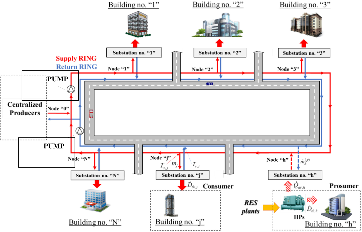
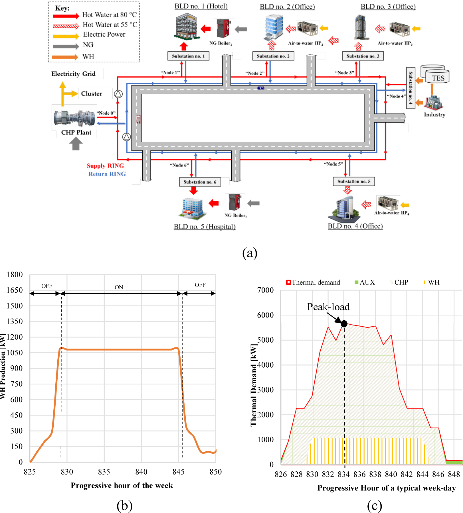
In Figure 1, simplified scheme of a ring-shaped heating network serving a cluster of buildings is shown. The red and blue lines indicate the supply (SR) and the return (RR) rings respectively. Numbered nodes are used to indicate the position of each substation along the grid. Worth noting that the possibility to have prosumers (e.g., Building no. “h”) is accounted for.
Ring-shaped network serving a cluster of buildings [23].
The thermohydraulic model of the network was obtained by applying mass and energy conservation to nodes, branches, and substations of the network. The water mass flow rate mj(τ) entering the j-th consumer’s substation at the time “τ” (e.g., seconds, hours, etc.) was calculated as follows:
(9)
where Dth,j is the thermal demand of the j-th consumer, is the specific heat of water, Ts,j and Tr,j are the supply line and return line temperature at the j-th building substation. Looking at the substation, it is possible to write:
(10)
where Usub and Asub are the overall heat transfer coefficient and the heat transfer area of heat exchangers in the substation. ΔTml is the logarithmic mean temperature difference between the water drawn from the substation and the temperature of the water returning from and supplied to the hydronic circuit of the user.
When considering water mass flow rate exchanged in the j-th node of the SR, it is possible to write:
(11)
where and are the water flow rate entering into and exiting the j-th node, respectively. is the mass flow rate supplied to SR by the j-th prosumer, and δC,j is a binary variable that describes the behavior of the j-th building as a “consumer” or “producer”. Indeed, when the building is a “consumer”, δC,j equals “1”, otherwise it equals “0”. Eq. (12) was used to calculate the mass flow rate taken from the RR, and supplied to the SR after being re-heated up within the substation,
(12)
Qav,h is the heat available from the h-th prosumer. Ts,nom is the nominal operating temperature of the SR. The value of Ts,nom is highly dependent on the generation of the considered DHN considered. If HPs are used by prosumers to supply heat to the network, the following equation can be used to calculate Qav,h(τ):
(13)
where COPHP,h is the coefficient of performance of the HP installed at h-th prosumer (either air-to water or water-to-water) and Pe,HP,h is the electric power consumed.
Once mass flow rates are found, distributed, and concentrated pressure drops Δpgrid in the grid are calculated via Eq. (14)
(14)
In Eq. 11, λk is the friction coefficient calculated by ad-hoc correlations, Dk is the diameter of the k-th tube of the grid, vk is the average velocity of the water, and Kt is a coefficient that depends on the type of concentrated pressure drop.
Regarding heat production, the thermal energy demanded by the network to the centralized heat producers, indicated here as Qtotal(τ) is calculated as follows:
(15)
where Qloss(τ) is the heat lost by the water circulating within the tubes and transferred to the ground. To calculate Qloss(τ), Eq. (16) can be used:
(16)
where Utube,k is the average heat transfer coefficient of the insulated tube of the k-th branch of the grid per unit length, Lk is the length of the tube, Tk is the temperature of the water within the tube, and Tsoil is the temperature of the soil.
As shown in Eq. (17), the thermal energy required by the network is then equal to the sum of energy available from k-th producers (e.g., CHP plants or WH). Worth noting that in the case of multiple energy producers, a coordinated share of Qtotal(τ) among producers must be formulated.
(17)
Finally, for the CHP plant, the fuel flow rate mfuel(τ) consumed during its operation would be calculated as follows:
(18)
where LHV is the Lower Heating Value of the fuel and ηth(TOD, PLR) is the thermal efficiency of the prime mover, which is a function of the temperature of the outdoor air TOD and the part-load ratio (PLR). PLR is the ratio of the heat delivered by the prime mover and the maximum value deliverable with a given TOD.
The electric power used to drive hydraulic pumps (more specifically, centrifugal pumps) in the network was calculated as:
(19)
where V(τ) is the volumetric flow rate, and ηp is the pump global efficiency.
In Figure 2, the productive structure of the thermal grid of Figure 1 is shown. The fuel, product, and residue (generated and allocated) are plotted. In Table 1, the equations used to calculate these exergy flows are detailed.
Productive structure of a ring-shaped thermal grid for exergy costing [23].
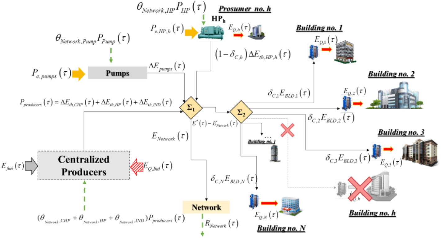
Fuel, Products, and Residues for a ring-shaped thermal network with multiple producers and prosumers
| Central producer | CHP plant | F | (20.a) |
| (20.b) | |||
| P | (20.c) | ||
| (20.d) | |||
| Industry | F | (20.e) | |
| P | (20.f) | ||
| Pumps | F | (g) | |
| P | (20.h) | ||
| Network (SR and RR) | F | (20.i) | |
| P | (20.j) | ||
| Building | Consumer | F | (20.k) |
| P | (20.l) | ||
| Producer | F | (20.m) | |
| P | (20.n) | ||
Regarding the centralized producer, the definition of the fuel depends on the adopted system. For a fossil-fueled CHP plant (e.g., gas turbines, combined cycles, etc.), the exergy content of the fuel supplied to the prime mover (indicated as Efuel) is usually identified as the exergy fuel. Meantime, two products could be identified: (i) the increase in the thermal exergy of the water supplied to the grid, indicated as ΔEth,CHP; and (ii) the delivered electrical power. Eqs. 20.a-n can be used to calculate these quantities. In Eq. 20.a, δ is a factor that is dependent on the type of fuel consumed [38], [39]. Moreover, Tref is the temperature of the reference environment (e.g., the outdoor air temperature or the temperature of the soil).
For the industrial process that supplies a WH flow to the network, the exergy content of the thermal energy QInd, k(τ) mind(τ)) heated up using QIND (indicated as ΔEth,IND(τ)) is considered as the useful product (Eq. 20.f).
Regarding pumps, the consumed electric power is the fuel (Eq. 20.g), and the increase in the exergy of water flow (i.e., ΔEpump(τ) in Eq. 20.h) is assumed as the product. Note that the exergy content of electric power is equal to the power itself according to [38].
The SR and RR rings destroy part of the exergy produced by the centralized plants and the pumps (ENetwork in Figure 2). This exergy destruction is due to heat losses and pressure drop, and according to ECT is considered as a residue (indicated as RNetwork, green arrows in Figure 2). Eq. 20.i was used to calculate this exergy destruction. Then, following the criterion proposed by Torres et al. [36], its exergy cost is allocated as additional fuel to the CHP plant, Industry, and pumps.
Regarding building substations, a different definition of fuel and product is adopted whether it is a producer or a consumer. In particular:
i-th Building as a consumer: the building consumes the exergy flow “EBLD,j” from the grid (eq. 20.k) to produce the exergy flow “EQ,j” of hot water used then for covering space heating and hot water demand (Eq. 20.l). Note that, in Eq. 20.k-l, exergy variation due to water temperature change and pressure drop are accounted for. Moreover, Ts,j, ps,j and Tr,j, pr,j are the temperature and pressure of SR and RR at j-th node. Tw.s and Tw,r are the temperature of water supplied and returning from the hydronic plant of the served building and mw, j is the water mass flow rate.
i-th Building as a producer: the exergy product ΔEth, HP,h is equal to the increase of the exergy of the flowrate from the temperature Tr,j (temperature of the j-th node on the RR) to Ts,n (Eq. 20.n). In the case of a prosumer equipped with HPs, the fuel is the electric power used to drive the HPs Eq. 20.m).
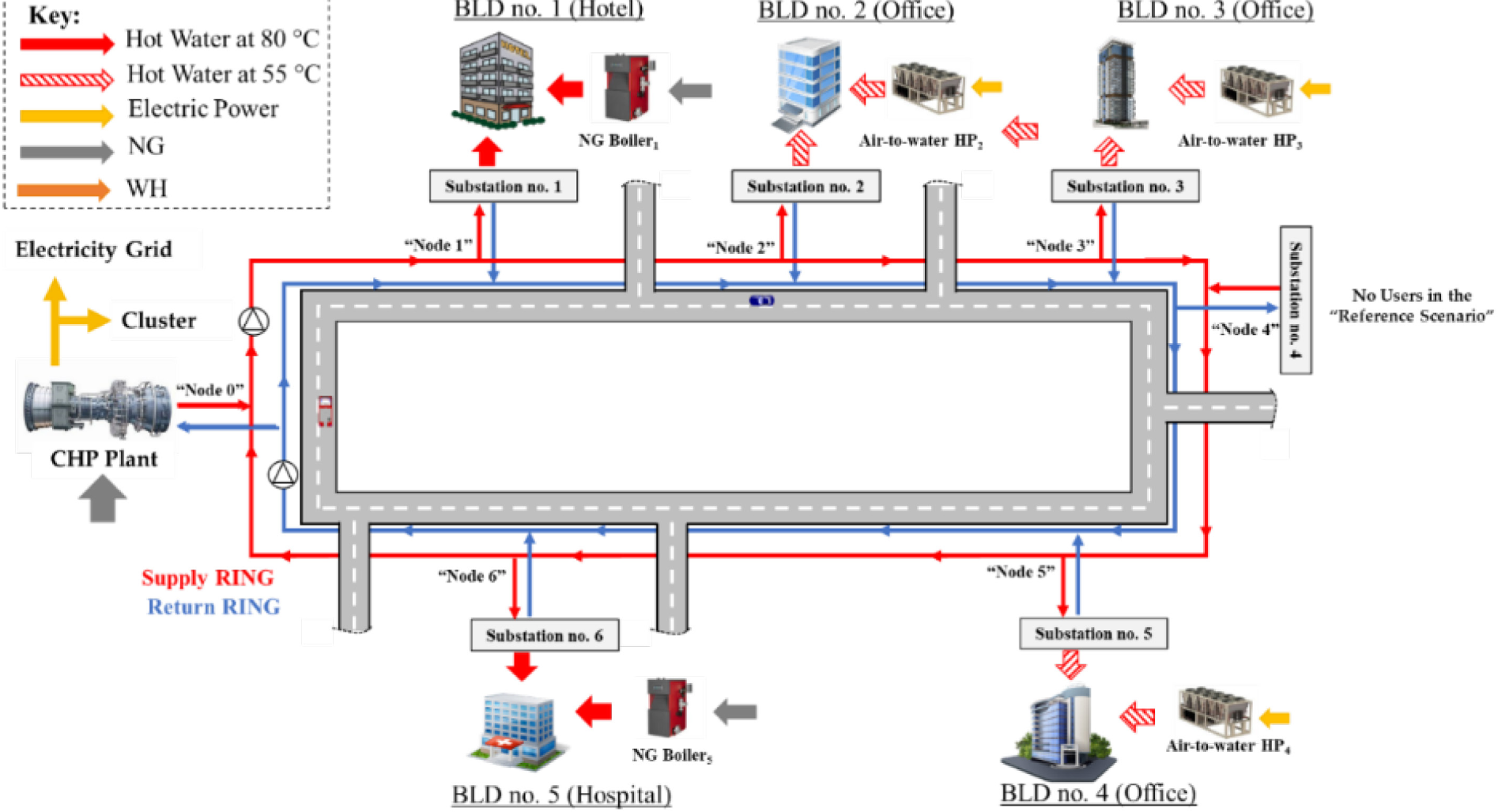
A cluster of five buildings (briefly indicated as BLD in the following) of the tertiary sector was considered as the case study (Figure 3). It was assumed that the cluster was in Sicily (Italy), and it consisted of the following BLDs: three offices, one hospital, and one hotel. In Table 2, distances among substations are reported. The peak value of the thermal demand of each BLD is also presented. As shown in Figure 3, air-to-water HPs or natural gas (NG) boilers were installed at each consumer not only to supply the uncovered part of thermal demands (for instance, in case of low thermal demand during night-time when it was not economically viable to operate the centralized plant) but also for the sake of redundancy. The nominal heating capacity of local generators is shown in Table 2.
Main data of the thermal grid and substations.
| Length [m] | Peak of Thermal Demand | Substations UA[kW/°C] | Local Heat Generator | ||||
|---|---|---|---|---|---|---|---|
| Type and number | HC* [kW] | COP* [-] | |||||
| Branch 0-1 | 300 | BLD no. 1 | 1520 | 172.65 | NG Boiler (no. 4) | 391 | - |
| Branch 1-2 | 375 | BLD no. 2 | 750 | 30.40 | Air-to-Water HPs (no. 2) | 421 | 3.07 |
| Branch 2-3 | 275 | BLD no. 3 | 1100 | 40.60 | Air-to-Water HPs (no. 3) | 421 | 3.07 |
| Branch 3-4 | 400 | BLD no. 4 | 490 | 19.86 | Air-to-Water HPs (no. 2) | 276 | 3.21 |
| Branch 4-5 | 250 | BLD no. 5 | 2210 | 303.67 | NG Boiler (no. 5) | 451 | - |
| Branch 5-6 | 250 | CHP Plant | - | 67.39 | - | - | - |
| Branch 6-0 | 300 | Industry | - | 43.14 | - | - | - |
Heating capacity and COP of the HPs refers to the following boundary conditions: variation of the water temperature in the condenser from 40 to 45 °C; an outdoor dry air temperature equal to 7 °C; outdoor air wet bulb temperature equal to 6 °C.
Regarding substations, the UA values are reported in Table 1. These values were calculated according to Eq. 7, by considering an operating temperature of the SR equal to 85 °C and a minimum temperature difference among the water flow drawn from the network and water circulating in the hydronic loop of the building equal to 5 °C. In this respect, the hot water produced in the substations was not the same for all BLDs. For BLD no. 1 and BLD no. 5, it was assumed that water returning from the hydronic circuit was heated up to 78-80 °C. For BLDs no. 2-3-4, instead, hot water at 55 °C was produced. NG gas turbines (GT) were assumed as prime movers in the CHP plant (located in “Node 0” in Figure 3). Moreover, the SR was operated at 85 °C as in the case of 3rd generation of DHNs. The UA value of the CHP plant substation is also reported in Table 2.
Scheme of the cluster of five buildings considered as the case study.
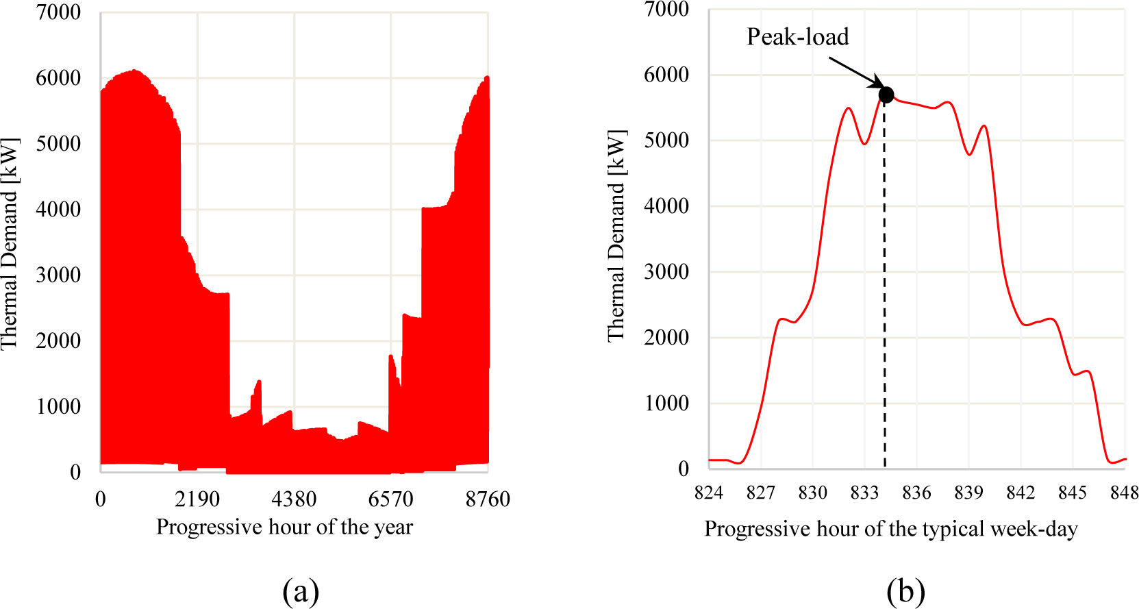
In Figure 4.a, the overall thermal demand of the cluster is shown. The thermal demand profile was derived from a previous study [40]. A peak of around 6.1 MWth was observed. Moreover, in Figure 4.b, the hourly profile of a typical weekday in winter (beginning of February) is shown. According to the methodological scope of this paper, the following analysis will focus only on the exergy cost analysis for the peak hour in the considered day (indicated by the black dot in Fig 4.b). More specifically, the peak value was around 5,690 kWth.
Thermal demand of the cluster for the (a) annual profile and (b) typical week-day profile.
As previously clarified, for the case study it was assumed a NG-fueled GT as a CHP plant which supplies heat to the heating network, and the SR was operated at 85 °C. This condition will be indicated in the following as the Reference Scenario. To show the capabilities of ECT, three alternative scenarios were investigated and compared with the reference one. In particular:
Scenario no. 1. It was assumed to supply the network not only by a CHP plant but using also a low-temperature WH flow (LT-WH) at 110 °C available from an industrial process (located in “Node 4” of the network in Figure 5.a). The operating temperature of the SR was equal to 85 °C, as in the reference scenario. Regarding the LT-WH profile production, the profile shown in Figure 5.b was assumed. Note that WH is produced simultaneously with the industry operation (this time frame is indicated by “ON” in Figure 5.b). Moreover, as shown by Figure 5.c, it was assumed that the LT-WH was produced almost during the whole daytime. Fig. 5.c depicts the contribution of the CHP plant and LT-WH in meeting the thermal demand. “AUX” refers to the energy supplied by local heat generators.
Scenario no. 2. The operating temperature of the network was lowered down to 60 °C as in the case of 4th Generation DHNs. The LT-WH was also assumed to supply the network. However, in this case, to supply BLDs no. 1 and 5, booster HPs (i.e., water-to-water HP) were included within substations to achieve the hot water temperature required by the building.
Scenario no. 3. It was assumed to lower the operating temperature to 45 °C to exploit the heat available from prosumers. More specifically, it was assumed that to help the power grid operator in managing electricity surplus from RES, BLD no. 2 and 4 activated their air-to-water HP instead of buying heat from the grid. Moreover, since it was assumed to operate the HPs at their maximum capacity, the surplus heat produced onsite is sold to the network. Referring to the day shown in Figure 4.b, by comparing the heating demand of BLDs no. 3 and 4 and the heating capacity of air to water HP, it was found that about 153 kWth and 131 kWth of thermal power could be supplied by the BLDs no. 3 and 4, respectively. Finally, due to the reduced operating temperature of the network, booster HPs were included in all building substations to achieve the temperature required by these users. Differently from Scenarios no. 1 and 2, no LT-WH was included here.
Worth noting that a profile like the one shown in Figure 5.c was developed for Scenario no. 3 as well, but not shown here for the sake of brevity.
Scenario no. 1: (a) position of the industry along the grid; (b) LT-WH production profile, and (c) demand covered by the CHP plant, WH and local heat generators.
Two small GTs (fueled by NG) with a nominal electrical and thermal capacity equal to 2.35 MWe and 3.7 MWth each are assumed to be installed. Worth noting that the overall nominal capacity of the CHP plant (i.e., 7.4 MWth) is greater than the peak of the thermal demand shown in Figure 4.a (i.e., 6.1 MWth). The selection was made considering a 7.3 MWth peak of the “aggregated thermal demand” (which was found by assuming the possibility to cover the overall cooling demand by using absorption chillers installed at each user substation with an average COP=0.7 [41]). Eqs (21) and (22) were adopted to calculate the thermal and electrical efficiency of the GT when operating at part load.
(21)
(22)
where PLR accounts for the full- and part-load operation. These curves were developed based on data available in [42] at different TOD values. A decrease in the energy performance of the prime mover is observed when the GT operates at PLR lower than one.
Regarding the COP of air-to-water HPs installed on BLDs, performance curves developed by the authors in another study were used [43]. Regarding the COP of the booster HPs, the performance curves available in [44] were used.
Regarding the temperature of the reference environment for exergy calculation (i.e., Tref), the temperature of the outdoor air was assumed.
The thermohydraulic and the exergy cost modeling presented in Section 2 were jointly solved using Engineering Equation Solver (EES) [45]. Note that the following assumptions were made:
The inner tube diameter of the grid was selected limiting the value of the average pressure drop per unit length of the grid in the range 150-250 Pa/m. The nominal diameter of a pre-insulated steel pipe that satisfied this condition was 180 mm, with a linear heat transfer coefficient Utube equal to 0.4 W/(m·°C).
The electricity used to drive the HPs’ prosumers was assumed to be produced by using electricity from RES plants.
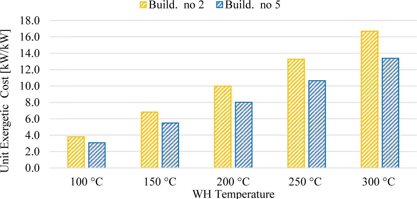
The following sensitivity analyses were performed only for Scenario no. 1:
first, the sensitivity of the unit exergetic cost of the heat with the WH temperature was investigated; more specifically, by assuming the same hourly WH amount (i.e., 1,080 kWh, see Figure 5.b) the following temperatures were considered: 100-150-200-250 and 300 °C.
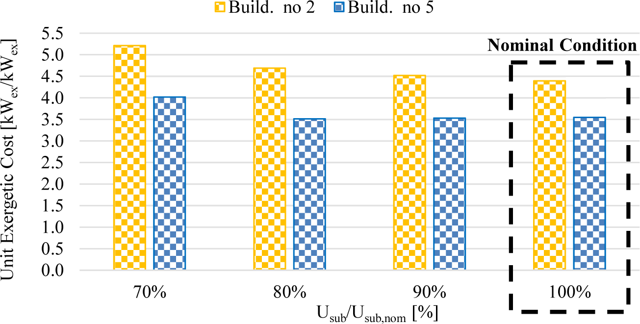
the effect of substation maintenance on the unit exergetic cost of heat was evaluated. In the case of poor maintenance, a progressive decrease in the heat exchanger properties (more specifically in the Usub) is observed. According to Eq. (10), to exchange the same amount of heat and to compensate for a reduced Usub, a greater logarithmic mean temperature difference is required. Then, according to Eq. (10) an increase in the amount of water drawn by the substation from the grid is consequent. Referring to the substation of BLDs no. 2 and no. 5, it was assumed a 5-10-20 % reduction of the overall heat transfer coefficient.
In the following subsections, results are separately shown and discussed for each scenario. After that, a comparative analysis is performed. In the last part of this section, the results of the sensitivity analyses are presented.
The results of the exergy cost analysis for the reference scenario are shown in Figure 6.a - b. The unit exergetic consumption values shown in Figure 6.a highlighted that the CHP plant is the one characterized by the highest exergy destruction. Moreover, the unit exergy consumption of substation in BLD. no. 2 is 25.8% higher than the one of BLD. no 5 due to the higher temperature difference between the temperature of water drawn from the SR and the one the hot water produced.
Results of the exergy cost analysis for the Reference Scenario: (a) unit exergy consumption, and (b) unit exergetic cost.
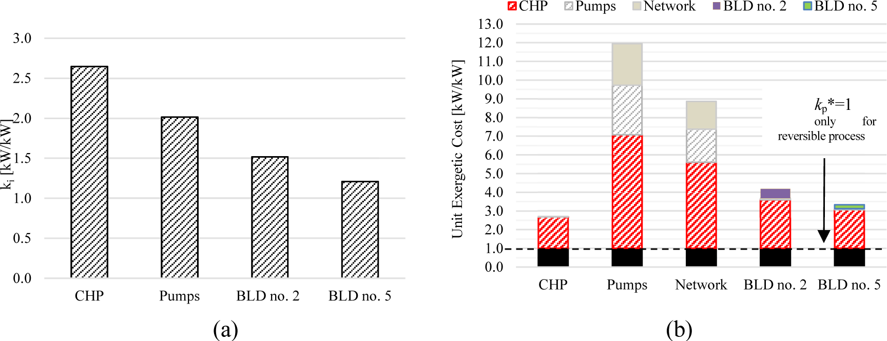
The unit exergy cost values are shown in Figure 6.b. Regarding the unit exergetic cost of the heat supplied to the BLDs, kp*, a value of 3.29 kWex/kWex was found for BLD no. 5 and 4.15 kWex /kWex for BLD no. 2. The decomposition of the unit exergy cost of the heat supplied to the users (as shown by the different colored bars in Figure 6.b) show that irreversibility generated by the CHP plant (red striped area) play a key role in determining the final unit cost. The irreversibility generated with substation slightly contributes to the final exergy cost of BLD no. 2, conversely, its contribution is negligible for BLD no. 5. The irreversibility generated in the pumps and in the network does not affect the unit exergetic cost of the heat supplied to the buildings.
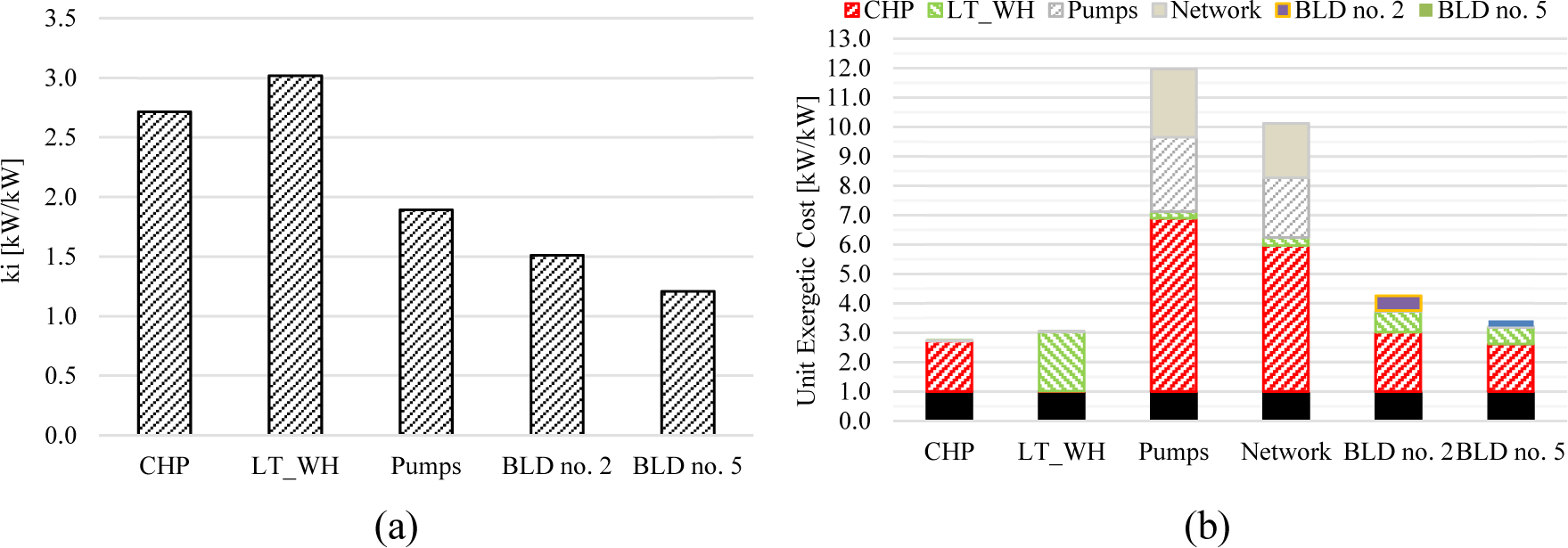
The results of the exergy analysis for this scenario are shown in Figure 7.a-b. As shown in Figure 7.a, the unit exergy consumption of the CHP plant increases from 2.65 up to 2.72 kWex/kWex when passing from the Reference to Scenario no. 1 (+2.64%). Such a result is a consequence of the part-load operation of the CHP. Indeed, since a fraction of the thermal demand is covered using WH from the industry, the CHP plant operates at part load. In this case, according to Eqs (21) and (22), the energy performance (and then the exergy performance) of the CHP plant decreases. Looking at Figure 7.a, it is possible to observe that a high exergy destruction occurs the in substation aimed at the recovery of the WH. Regarding the unit exergy cost of the heat supplied to the buildings, kp*, as shown in Figure 7.b, a value of 4.36 kWex/kWex was found for BLD no. 2 and 3.50 kWex /kWex for BLD no. 5. The decomposition of the unit exergy cost of the heat supplied to the users shows that also in this case, the irreversibility generated within the CHP plant (red area) plays a key role in determining the final unit cost (more than 50%). Then, the irreversibility generated in the recovery of the WH (green area) affects the unit exergetic cost of the heat supplied by about 24% in the case of BLD no.2, and 6.6% in the case of BLD no. 5. Finally, the exergy destruction in substations moderately contributes to the final exergetic cost.
Results of the exergy cost analysis for Scenario no. 1: (a) unit exergy consumption, and (b) unit exergetic cost.
The results for Scenario no. 2 are shown in Figure 8.a-b. Note that due to the installation of the booster-HPs in BLDs no. 1 and 5, almost a 50% reduction of the heat demanded by the grid to centralized producers (i.e., CHP plant and the industry) is estimated with respect to Scenario no. 1. In this case, the CHP plant is operated at a lower PLR compared to Scenario no 1, and an increase in the unit exergy consumption of the CHP plant (Figure 7.a) is observed passing (+66%). Moreover, an increase in the unit exergy consumption in the WH recovery is found when comparing Scenarios no. 1 and no. 2, due to the larger average temperature difference between the WH temperature (110 °C) and the SR temperature (60 °C).
Results of the exergy cost analysis for Scenario no. 2: (a) unit exergy consumption, and (b) unit exergetic cost.
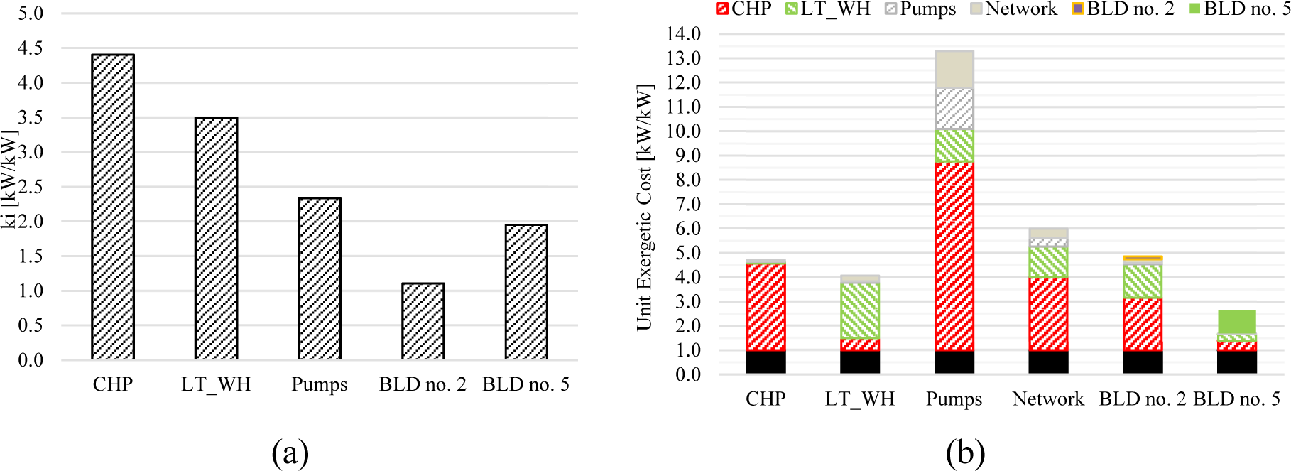
Regarding the unit exergetic cost of the heat supplied to the BLDs (shown in Figure 8.b), it is possible to observe that it increases up to 4.84 kWex /kWex for BLD no. 2 and it decreases down to 2.63 kWex/kWex for BLD no. 5. Moreover, worth noting that the unit exergetic cost of BLD no. 2 is highly influenced by the irreversibility occurring in the CHP plant and LT-WH substation. Regarding BLD no. 5, although the exergy destruction in the substation is increased due to the presence of the booster-HP (blue area), the reduction of the thermal exergy drawn from the network leads to a reduction in the unit exergetic cost.
In this scenario, it was assumed that due to the surplus of RES electricity in the power grid, HPs in BLD no. 3 and no. 4 were operated at their maximum capacity, and the exceeding heat was provided to the heating network (thus becoming prosumers). In Figure 9, the exergy unit cost values are shown. Worth noting that for BLD no. 2, the unit exergetic cost decreased to 2.98 kWex/kWex (almost -38.4% with the one obtained in Scenario no. 2) thanks to the insertion of the booster HP. The unit exergetic cost of heat supplied to BLD no. 5, decreased from 2.93 (Scenario no. 2) to 2.19 in Scenario no. 3 (-25.2%). Moreover, in this scenario, the unit exergetic cost of heat supplied to BLDs no. 2 and 5 is more sensitive to the inefficiencies occurring in the substation than the one occurring in the CHP plant. Finally, it is worth noting that the effects of inefficiencies occurring in the prosumers (the BLDs no. 3 and no. 4) on the unit cost of the heat supplied to BLDs no. 2 and no. 5 are negligible.
Results of the exergy cost analysis for Scenario no. 3: unit exergetic cost.
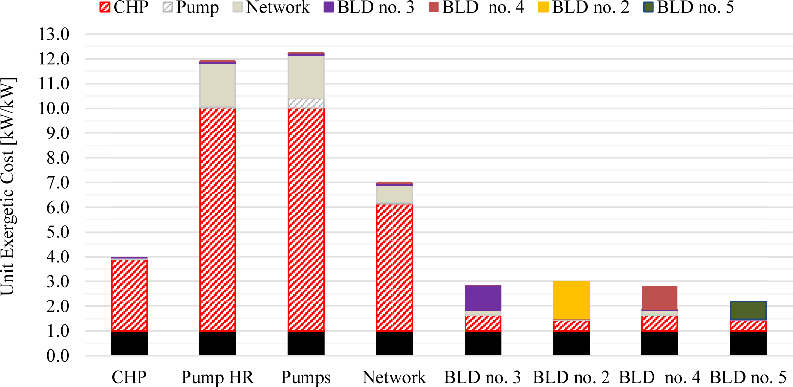
Table 3 collects the unit exergetic cost of the heat supplied to BLDs no, 2 and no. 5 for all proposed scenarios. Moving from the Reference Scenarios to Scenario no. 1, the unit exergetic cost increases by about +5.5%. This increase testified that the inclusion of the assumed amount of WH at 110 °C does not lead to a great improvement in the thermodynamic efficiency of the grid. Passing to Scenario no. 2, a further increase in the unit exergetic cost of the heat supplied to BLD no. 2 is observed, meaning that although the lower operating temperature of the network reduces heat losses along the network, this does not lead to an increase of the overall thermodynamic efficiency. Worth noting that a reduction in the unit exergetic cost of the heat supplied to BLD no. 2 could be achieved in Scenario 2, only in the case of LT-WH if a temperature lower than 110 °C would be available. When moving to Scenario no. 3, thanks to the insertion of booster HP and the use of heat coming from prosumers, a substantial decrease in the unit exergetic cost is observed.
Unit Exergetic cost of heat supplied to the representative BLDs.
| kp* [kWex /kWex] | Reference Scenario | Scenario no. 1 | Scenario no. 2 | Scenario no. 3 |
|---|---|---|---|---|
| BLD no. 2 | 4.15 | 4.36 (+5.1%) | 4.84 (+16.6%) | 2.98 (-28.2%) |
| BLD no. 5 | 3.29 | 3.50 (+6.4%) | 2.63 (-20.1%) | 2.19 (-33.4%) |
As previously clarified, the first sensitivity analysis investigated for Scenario no. 1 is the effect of the temperature of the WH on the unit exergy cost of the heat. More specifically, the WH temperature was varied from 100 °C up to 300 °C. The results of this analysis are shown in Figure 10. Note that when the WH temperature is increased, the unit exergy cost of the heat steeply increases. For instance, for BLD no. 2, the unit exergetic cost increases from 3.80 kWex/kWex when a WH flow at 100 °C is assumed, up to 16.69 kWex/kWex for the WH at 300 °C. This large variation in the unit exergetic cost of the heat suggested that the use of medium-temperature WH flows for producing low-temperature hot water within building substations is not rational.
Results of the sensitivity analysis of the unit exergy cost of the heat with the temperature of the WH flow.
The second sensitivity analysis investigated the effect of substations’ maintenance on the unit exergetic cost of the heat supplied to the considered buildings. Results are shown in Figure 11. Note that, when the Usub value is reduced from 100% to 80%, a gradual increase in the unit exergetic cost of heat for BLD no. 2 is observed (+6.83%). However, when Usub is decreased from 80% to 70% of the nominal value (which would occur in the case of very poor maintenance) a higher change in the unit exergy consumption is observed (+18.5%). Regarding the unit exergy cost of heat supplied to BLD no. 5, it is possible to observe that its value is not sensitive to off- design operation in the substation on BLD no. 2, in case of a low and moderate reduction in Usub. However, in case of a heavy reduction of Usub, also the unit exergy cost of heat supplied to BLD no. 5 increases. This result is very important as it shows that this indicator could allow for the prediction of off-design operations of substations and then support the scheduling of proper maintenance programs.
Results of the sensitivity analysis of the unit exergy cost of the heat with the maintenance of the substations in BLDs no. 2 and no. 5.
This work proposed ECT for supporting the design and operation of heating networks serving a cluster of buildings. To show the capabilities of this method, a cluster of five buildings in the tertiary sector was assumed as the case study. Some scenarios were compared, respectively characterized by a centralized GT-based CHP plant, the integration of WH, and the presence of prosumers. Results demonstrated that the use of unit exergetic cost of heat could help identify which steps along the heat production process highly contribute to lowering the thermodynamic efficiency, and then leading to high operating costs. More specifically, from this analysis, it was found that the inefficiencies occurring in the CHP plant accounted for almost 50% of the unit exergy cost of the heat supplied to the buildings. Moreover, it was found that a lower operating temperature of the network did not lead to better thermodynamic efficiency if the same heat production units were assumed to supply the network, by keeping the same systems for heat generation. Finally, the analysis revealed a 30% reduction in unit exergy cost of heat when moving from a centralized to a decentralized production, although booster HPs should be installed within substations, The proposed model was useful for performing sensitivity analyses. For instance, when the WH temperature increases, the unit exergy cost of the heat consumed by buildings steeply increases because of the higher exergy destruction occurring in the substation. This trend justified the poor rationale for using medium-temperature WH for space heating. Moreover, in case of poor maintenance in building substations, the increasing value of unit exergy cost of the heat provided not only a quantitative assessment of extra resources consumed for heat production in the off-design condition but also a support for scheduling of proper maintenance program. In conclusion, ECT could provide support in the design, operation, and monitoring of thermal grids.
This study was developed in the framework of the research activities carried out within the Project “Network 4 Energy Sustainable Transition—NEST”, Spoke 7: Smart Sector Integration, Project code PE0000021, funded under the National Recovery and Resilience Plan (NRRP), Mission 4, Component 2, Investment 1.3—Call for tender No. 1561 of 11.10.2022 of Ministero dell’Università e della Ricerca (MUR); funded by the European Union— NextGenerationEU.
- , , World Energy Outlook 2022, 2022
- ,
Smart Energy Systems for Coherent 100% Renewable Energy and Transport Solutions ,Appl Energy , Vol. 145 ,pp 139–154 , 2015, https://doi.org/https://doi.org/10.1016/j.apenergy.2015.01.075 - ,
Impact of Renewable Energy Expansion to the Balancing Energy Demand of Differential Balancing Groups ,Journal of Sustainable Development of Energy, Water and Environment Systems , Vol. 6 ,pp 784–799 , 2018, https://doi.org/https://doi.org/10.13044/j.sdewes.d6.0215 - ,
Stability Enhancement of a Power System Containing High-Penetration Intermittent Renewable Generation ,Journal of Sustainable Development of Energy, Water and Environment Systems , Vol. 3 ,pp 151–162 , 2015, https://doi.org/https://doi.org/10.13044/j.sdewes.2015.03.0012 - ,
Technical, Economic, and Environmental Assessment of Integrating Solar Thermal Systems in Existing District Heating Systems under Jordanian Climatic Conditions , Vol. 10 , 2022, https://doi.org/https://doi.org/10.13044/j.sdewes.d9.0395 - ,
Industrial Waste Heat: Estimation of the Technically Available Resource in the EU per Industrial Sector, Temperature Level and Country ,Appl Therm Eng , Vol. 138 ,pp 207–216 , 2018, https://doi.org/https://doi.org/doi.org/10.1016/j.applthermaleng.2018.04.043 - ,
Waste Heat from Data Centers: An Investment Analysis ,Sustain Cities Soc , Vol. 44 ,pp 428–444 , 2019, https://doi.org/https://doi.org/10.1016/j.scs.2018.10.023 - ,
V Review and Validation of EnergyPLAN ,Renewable and Sustainable Energy Reviews , Vol. 168 ,pp 112724 , 2022, https://doi.org/https://doi.org/10.1016/j.rser.2022.112724 - ,
Energy Mapping and District Heating as Effective Tools to Decarbonize a City: Analysis of a Case Study in Northern Italy ,Energy Reports , Vol. 7 ,pp 254–262 , 2021, https://doi.org/https://doi.org/10.1016/j.egyr.2021.08.147 - ,
International Review of District Heating and Cooling ,Energy , Vol. 137 ,pp 617–631 , 2017, https://doi.org/https://doi.org/10.1016/j.energy.2017.04.045 - ,
4th Generation District Heating (4GDH): Integrating Smart Thermal Grids into Future Sustainable Energy Systems ,Energy , Vol. 68 ,pp 1–11 , 2014, https://doi.org/https://doi.org/10.1016/j.energy.2014.02.089 - ,
5th Generation District Heating and Cooling Systems: A Review of Existing Cases in Europe ,Renewable and Sustainable Energy Reviews , Vol. 104 ,pp 504–522 , 2019, https://doi.org/https://doi.org/10.1016/j.rser.2018.12.059 - ,
Perspectives on Fourth and Fifth Generation District Heating ,Energy , Vol. 227 ,pp 120520 , 2021, https://doi.org/https://doi.org/10.1016/j.energy.2021.120520 - ,
The Four Generations of District Cooling - A Categorization of the Development in District Cooling from Origin to Future Prospect ,Energy , Vol. 253 ,pp 124098 , 2022, https://doi.org/https://doi.org/10.1016/j.energy.2022.124098 - ,
District Heating Network Design and Configuration Optimization with Genetic Algorithm ,Journal of Sustainable Development of Energy, Water and Environment Systems , Vol. 1 ,pp 291–303 , 2013, https://doi.org/https://doi.org/10.13044/j.sdewes..2013.01.22 - ,
Experimental Characterization of a Prototype of Bidirectional Substation for District Heating with Thermal Prosumers ,Energy , Vol. 223 ,pp 120036 , 2021, https://doi.org/https://doi.org/10.1016/j.energy.2021.120036 - ,
Dynamic Modeling of Local District Heating Grids with Prosumers: A Case Study for Norway ,Energy , Vol. 151 ,pp 261–271 , 2018, https://doi.org/https://doi.org/10.1016/j.energy.2018.03.033 - ,
Economic Comparison of 4GDH and 5GDH Systems – Using a Case Study ,Energy , Vol. 238 ,pp 121613 , 2022, https://doi.org/https://doi.org/10.1016/j.energy.2021.121613 - ,
A Dynamic Price Model Based on Levelized Cost for District Heating ,Energy Ecol Environ , Vol. 4 ,pp 15–25 , 2019, https://doi.org/https://doi.org/10.1007/s40974-019-00109-6 - ,
Thermo-Economic Optimization of a Hybrid Solar District Heating Plant with Flat Plate Collectors and Parabolic Trough Collectors in Series ,Energy Convers Manag , Vol. 165 ,pp 92–101 , 2018, https://doi.org/https://doi.org/10.1016/j.enconman.2018.03.034 - ,
Identification of Key Performance Indicators and Complimentary Load Profiles for 5th Generation District Energy Networks ,Appl. Energy , Vol. 291 ,pp 116672 , 2021, https://doi.org/https://doi.org/10.1016/j.apenergy.2021.116672 - ,
Thermoeconomic Cost Assessment in Future District Heating Networks ,Energy , Vol. 117 ,pp 485–491 , 2016, https://doi.org/https://doi.org/10.1016/j.energy.2016.07.016 - ,
Exergoeconomics as a Cost- Accounting Method in Thermal Grids with the Presence of Renewable Energy Producers ,Sustainability , Vol. 14 (7), 2022, https://doi.org/https://doi.org/10.3390/su14074004 - ,
Automatic Fouling Detection in District Heating Substations: Methodology and Tests ,Appl Energy , Vol. 258 ,pp 114059 , 2020, https://doi.org/https://doi.org/10.1016/j.apenergy.2019.114059 - ,
Fault Detection in District Heating Substations ,Appl Energy , Vol. 157 ,pp 51–59 , 2015, https://doi.org/https://doi.org/10.1016/j.apenergy.2015.07.061 - ,
System-Level Fouling Detection of District Heating Substations Using Virtual-Sensor-Assisted Building Automation System ,Energy , Vol. 227 ,pp 120515 , 2021, https://doi.org/https://doi.org/10.1016/j.energy.2021.120515 - ,
A Thermodynamic Analysis of a Novel Bidirectional District Heating and Cooling Network ,Energy , Vol. 144 ,pp 20–30 , 2018, https://doi.org/https://doi.org/10.1016/j.energy.2017.11.122 - ,
Economical, Environmental and Exergetic Multi- Objective Optimization of District Heating Systems on Hourly Level for a Whole Year ,Appl Energy , Vol. 251 ,pp 113394 , 2019, https://doi.org/https://doi.org/10.1016/j.apenergy.2019.113394 - ,
The Exergy Cost Theory Revisited ,Energies (Basel) , Vol. 14 (6),pp 1594 , 2021, https://doi.org/https://doi.org/10.3390/en14061594 - ,
Thermoeconomic Optimization of a Dual-Purpose Power and Desalination Plant ,Desalination , Vol. 136 ,pp 147–158 , 2001, https://doi.org/https://doi.org/10.1016/S0011-9164(01)00177-1 - ,
Depletion of the Non-Renewable Natural Exergy Resources as a Measure of the Ecological Cost ,Energy Convers Manag , Vol. 43 ,pp 1149–1163 , 2002, https://doi.org/https://doi.org/10.1016/S0196-8904(02)00005-5 - ,
Thermo-Ecological Cost of Electricity from Renewable Energy Sources ,Renew Energy , Vol. 115 ,pp 87–96 , 2018, https://doi.org/https://doi.org/10.1016/j.renene.2017.07.074 - ,
On Thermoeconomic Diagnosis of a Fouled Direct Expansion Coil: Effects of Induced Malfunctions on Quantitative Performance of the Diagnostic Technique ,Journal of Sustainable Development of Energy, Water and Environment Systems , 2016, https://doi.org/https://doi.org/10.13044/j.sdewes.d5.0141, N/A - ,
A Nearly Net-Zero Exergy District as a Model for Smarter Energy Systems in the Context of Urban Metabolism ,Journal of Sustainable Development of Energy, Water and Environment Systems , Vol. 5 ,pp 101–126 , 2017, https://doi.org/https://doi.org/10.13044/j.sdewes.d5.0136 - , The Thermodynamic of Cost Formation. In Exergy, Energy, Energy System Analysis and Optimization, Encyclopedia Life Support Systems, 2009
- ,
On the Cost Formation Process of the Residues ,Energy , Vol. 33 ,pp 144–152 , 2008, https://doi.org/https://doi.org/10.1016/J.ENERGY.2007.06.007 - , Symbolic Thermoeconomic Analysis of Energy Systems. In Exergy, Energy, Energy System Analysis and Optimization– Vol. II, Encyclopedia of Life Support Systems (EOLSS), 2009
- , , The Exergy Method of Thermal Plant Analysis, Butterworths, 1985
- , , Advanced Engineering Thermodynamics, 2016
- ,
A Comprehensive Tool for Efficient Design and Operation of Polygeneration-Based Energy Μgrids Serving a Cluster of Buildings. Part II: Analysis of the Applicative Potential ,Appl Energy , Vol. 111 ,pp 1222–1238 , 2013, https://doi.org/https://doi.org/10.1016/j.apenergy.2012.11.079 - ,
An Original Multi-Objective Criterion for the Design of Small-Scale Polygeneration Systems Based on Realistic Operating Conditions ,Appl Therm Eng , Vol. 28 ,pp 2391–2404 , 2008, https://doi.org/https://doi.org/10.1016/j.applthermaleng.2008.01.017 - , TRNSYS 17: A Transient System Simulation Program, Solar Energy Laboratory, 2010
- ,
Assessing the Energy- Saving Potential of a Dish-Stirling Con-Centrator Integrated Into Energy Plants in the Tertiary Sector ,Energies , Vol. 14 , 2021, https://doi.org/https://doi.org/10.3390/en14041163 - ,
Steady State Behavior of a Booster Heat Pump for Hot Water Supply in Ultra-Low Temperature District Heating Network ,Energy , Vol. 237 ,pp 121528 , 2021, https://doi.org/https://doi.org/10.1016/j.energy.2021.121528 - , , Engineering Equation Solver