


The demand for space cooling has increased dramatically in the past few decades, which significantly affects the electrical energy usage. In Abu Dhabi city, located in the western part of the United Arab Emirates between latitudes 22°40’ and about 25° north and longitudes 51° and about 56° east, the cooling demand consumption has increased in 2016 to reach approximately 70-75% of the total energy consumption, particularly during the summertime [1]. In general, the increase in energy consumption in buildings has been addressed as a major concern towards global warming all over the world. The Abu Dhabi Statistical yearbook [2] highlighted the climate as well as the water and electricity concerns. Despite the advanced development of air-conditioning systems, the use of energy by this sector is nearly uncontrolled and rapidly increases as a direct impact of global warming. Accordingly seeking a real solution to this dilemma is crucial and critical.
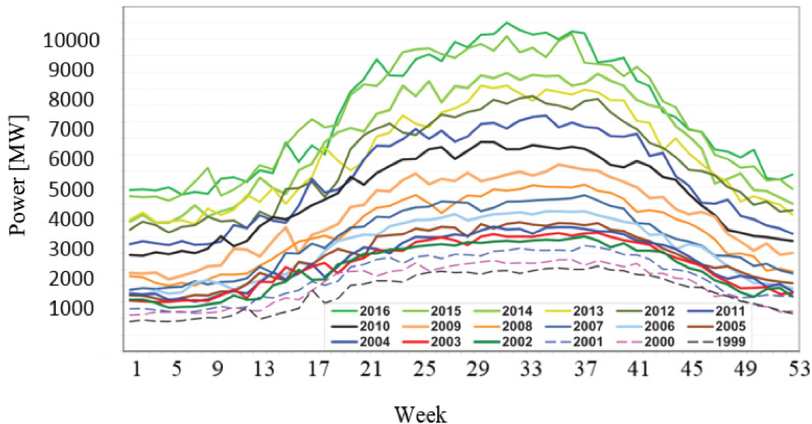
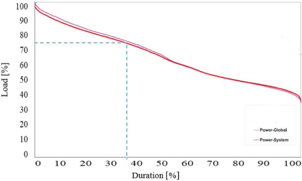
Figure 1 shows the electrical power loads at the peak time between 1999 and 2016 in Abu Dhabi averaged on weekly basis. The inflation of peak loads in the power sector burdens the generation authorities. In addition to the inflation in the peak loads, the part loads on both sides of the curves represent the winter and spring seasons. This duration of part load (less than 75% of full capacity) in 2016 was measured to be approximately more than 60% of the total year duration as shown in Figure 2.
Load forecasting model is employed to determine the size of power generation plants that are needed to satisfy the power demands. However, the instability in the power demand profile inversely affects the load forecasting accuracy.
Load curve of Abu Dhabi on 1999-2016 on weekly basis [1]
Percent duration of electrical load levels in 2016 [1]
The present study is addressing the feasibility of two control methods that can be implemented in a Chiller Cooling System (CCS) plant installed and commissioned recently in Masdar city in Abu Dhabi. The first method is adopting a control algorithm, which distributes the cooling load among multi-chillers that are initially connected in parallel inside the CCS plant. The second method is by using Thermal Energy Storage (TES) that stores chilled water for meeting the load during the demand peak hours. The thermal storage tank stores the chilled water during the off-peak hours and supplies it to the consumer-cooling load during the peak hours. Therefore, creating a possibility of lowering the chiller capacity, in addition to saving the cost resulting from the higher electrical power tariff during peak time.
Controlling a chiller cooling system plant is not a trivial task, where chillers, primary pumps, secondary pumps and cooling tower fans are involved, besides the instabilities in the cooling demand and the surrounding conditions. This complexity dramatically increases when the Variable Frequency Drive (VFD) technology is implemented in the electric motors driving pumps, fans, or compressors. Therefore, it enlarges the feasible region of the chiller loading optimization. In the literature, hundreds of optimization algorithms and techniques are proposed for optimum CCS operation. Some of these optimizations are uniquely feasible for only a particular cooling load profile whereas others are generally feasible for a wider range.
Huang et al. [3] have proposed three new approaches to Cooling Load-based Control (CLC) methods to optimize a CCS by investigating the pre-defined thermodynamic stages of chiller and condenser. Salari et al. [4] have also used CLC method for achieving an Optimal Chiller Loading (OCL) using a General Algebraic Modelling System (GAMS). Their results were in good agreement with other optimization techniques.
Wei et al. [5] optimized a CCS consisting of four chillers and two chilled water tanks, using a two-level algorithm to find the OCL. The tanks were charged and discharged at each time step based on the cooling load demand, and the electricity tariff. However, the optimization did not account for the tank losses during the time between charging and discharging. Moreover, Cuckoo optimization algorithm was used to optimize chillers-based plant only, where the algorithm was based on chiller consumption polynomial as a function of the Part Load Ratio (PLR) [6].
On the other hand, the temperature of the coolant into the condenser was considered in Chung optimization problem, where simulated annealing was implemented to find the optimal loading schedule for multi-chillers plant [7]. Others studied the supply chilled water temperature to find the OCL using Hopfield neural network in order to avoid any convexity in the feasible region [8].
Employing thermodynamic parameters of the vapour-compression-cycle has asignificant impact on the overall energy usage of the chiller. However, it is challenging to operate the chiller at optimal conditions due to the mechanical limitations of the components, environmental conditions, as well as, the load demand. A modified genetic algorithm was employed to determine the minimum energy consumption by the compressor, the condenser fan and the evaporator fan, and the results were compared to the normal on-off control strategy [9]. The simulation results showed about 8.45% energy saving achieved for a typical day. Determining the optimal operating conditions should also cover the superheated degree inside the evaporator, and the sub-cooled degree in the condenser. For this reason, Exergy-based optimization was developed to find the optimal areas for superheated and sub-cooled degrees [10].
Similar to CCS without TES, CCS plant that consists of multiple chillers and TES system does not work at constant loads all the time. Thus, it becomes necessary to determine an optimal loading scheme for not only the chillers but also for the CCS-TES system. Armstrong [11] performed a component-based optimization because the CCS components are coherent and work all together simultaneously. Different energy-saving approaches are investigated including a TES that is evaluated by annual cooling system energy consumption.
Recently, Model Predictive Control (MPC) optimization in CCS-TES system has been more widely used, in fact, the main challenge in this optimization method is to find a robust and optimal solution in the presence of integer and nonlinear constraints. Ma et al. [12] have proposed a simple model of CCS that is connected to a sensible TES storage unit. The model solves for the optimal chilled water return temperature and the water level inside the TES at each time-step using MPC. The Branch and Bound (BB) algorithm with moving window-blocking strategy is used to solve the Mixed Integer Nonlinear Program (MINLP) optimization problem.
Deng et al. [13] modelled an integrated CCS-TES system dynamically using a bilinear model, where MPC aimed to reduce the system electricity consumption without violating the cooling load’s constraints and the physical limitations. The MINLP optimization problem was solved by initiating an arbitrary loading profile for the TES alone in order to linearize the problem, then applying a dynamic programming method to solve for the MILP. Lu et al. [14] added a penalty on the chiller’s on/off sequence in the objective function, in which energy saving was confirmed using MINLP optimization.
TES technology modification was investigated by many researchers, where some investigate the stratification of the sensible TES by adding a phase change material capsulate to the tank [15], while others studied the impact of the TES location on the overall performance of the system [16]. Peak load shaving is also investigated to capture the cost saving when using time of use tariff [17]. However, as of our knowledge, none of the researchers has uniquely investigated the energy-saving potential of TES technology when integrated with a CCS.
TES technology is proposed to eliminate the effects of the two previously mentioned problems, namely: increasing the peak-load and working apart from the optimum operation point. This technology is coupled to a conventional chiller system that shaves the peak load and smooths the overall load simultaneously, seeking to eliminate part of the operating cost through working at lower electricity cost during off-peak hours (time-of-use tariff) in some countries. In countries where the electricity time-of-use tariffs are not employed, TES is rarely used, however, this paper aims to compare both technologies commonly adopted to CCS namely, the TES and CLC in a two-chillers plant. An experiment-based model is proposed to investigate the viability of adopting both technologies on CCS subjected to a hot and humid climate at a typical cooling load. The models are validated by experimental data from the Masdar CCS plant in order to accurately investigate the chiller operation performance, under both scenarios (CLC algorithm and TES tank). The TES operating strategy can be one of two known strategies, partial in which the tank is charged to meet the only portion of the load in a specific time (peak), or full in which the tank is charged to meet the total load in the specific time (peak). However, the partial load strategy is chosen here for its simplicity, and based on that, the size of the tank is calculated [18].
Chiller manufacturers usually design the chiller to be capable of meeting the maximum expected load, however, this maximum load is only required for specific days over the year, and selected hours during these days. Thus, chillers operate at a fraction of their own capacity most of the time, lowering their average Coefficient of Performance (COP), and increasing their energy consumption when operating without VFD technology. Although some designers try to overcome this problem by distributing the load on multiple small-capacity chillers, this gives rise to an increase in the chiller plant’s capital cost.
TES integration with a chiller cooling system can be useful in two situations. First, where electricity is available in different tariffs such that TES can be implemented to save the operating cost. Second, where the load is varying frequently with time so the TES can smooth the peak load subjected to the chillers, resulting in higher average COP and lower energy consumption, which is the focus of this paper.
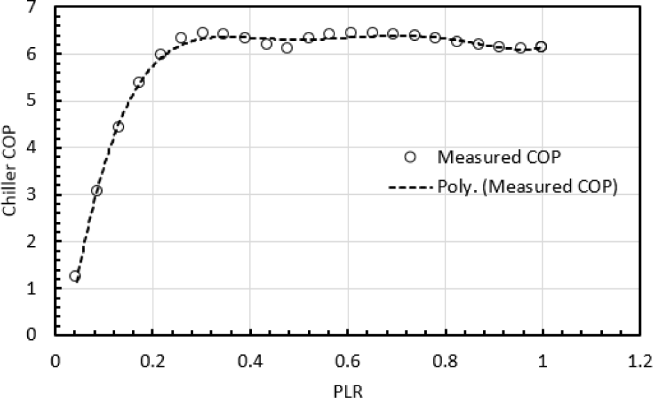
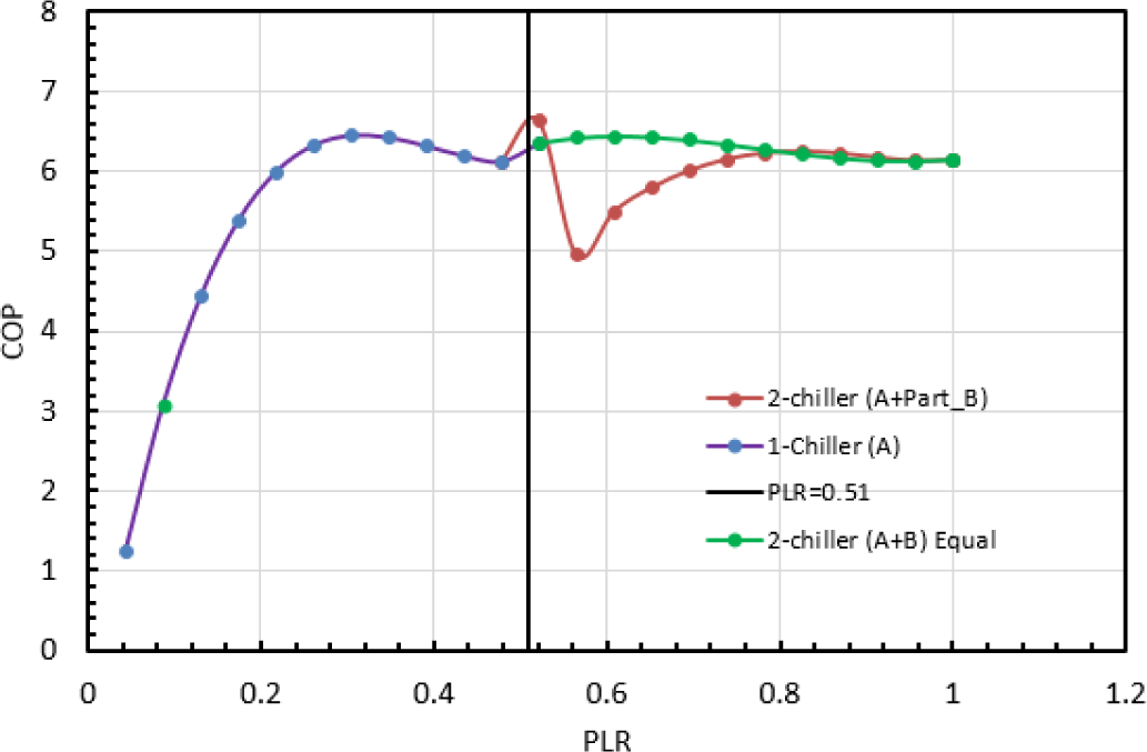
Two identical chillers in parallel forming a district cooling plant of a total capacity of 3,300 tons (11,600 kW) supply of chilled water at 7 °C are modelled using realistic data from the current operation. The data is utilized to determine the chillers’ electrical power as a normalized function of the demand load to the design load, or simply the PLR. The collected data is processed, after which the chiller COP is plotted against the PLR as shown in Figure 3. The COP plots for both chillers are curve-fitted and modelled by a fifth-order polynomial as illustrated in eq. (1), where chiller A and B have the same part load performance:
(1)
Chiller COP with PLR
In order to assess the true contribution of integrating the TES with CCS, three different scenarios are studied. First, scenario-I, involves chillers A (6,000 kW) and B (5,600 kW) without TES, functioning on equal load-control strategy whenever the system requires two chillers to meet the demand. Second, scenario-II, involves chiller A and B without TES. In this scenario, chiller A operates first to meet the cooling load, and chiller B operates only when cooling load exceeds the chiller A capacity. Thus, the remaining load will be taken care of by chiller B. Third, scenario-III, proposes an integration of a chilled water TES with the two chillers CCS plant aiming to operate the integrated system at the highest COP regardless of the cooling load.
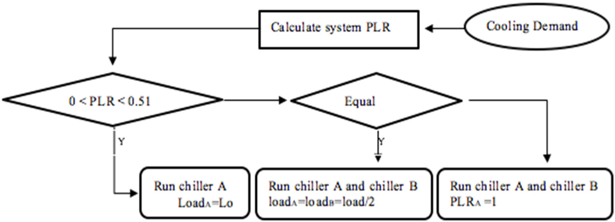
CLC algorithm as illustrated in Figure 4 is implemented in the first two scenarios for chiller loading controls. In this analysis, pumps, cooling tower fans, and air handling units are eliminated. The algorithm is applied to control the first two scenarios, where first the magnitude of cooling load would be used to calculate the PLR. Then if the PLR is in the range 0 to 0.51 (6,000/11,600), the load will be met by running chiller A only (in both scenarios). On the other hand, if PLR is in range of 0.51 to 1, the load will either be divided equally between A and B (scenario-I), or chiller A will run on full load and B on the remaining partial load (scenario-II) in order to satisfy the total demand.
The chiller’s needed power is obtained from eq. (2) for chiller A and eq. (3) for chiller B. The required energy in kWh for the cooling system is also obtained for one storage cycle (24 hours) using eq. (4):
(2)
(3)
(4)
where LoadA and LoadB are the cooling loads [kW], for chillers A and B respectively. PowerA and PowerB represent the electrical power [kW], of the two chiller’s compressors, respectively, and t is the storage cycle time measured in hours. In the third scenario, the method for the TES integration tank following partial strategy control is initiated by defining the demand peak and off-peak hours. Algorithm 1 is developed and implemented by assuming an initial guess for the off-peak period based on the cooling load profile, as shown in Figure 4. Then, an optimization framework is performed to deduce the optimal off-peak period. The TES tank is charged during the off-peak and is discharged during the peak period. Finally, the actual volume of the stratified chilled water tank is obtained using eq. (5).
Control algorithm for the two chillers cooling system without energy storage
Algorithm 1: Determination method for optimal partial storage tank (sensible) capacity
 |
After determining the tank and the chiller capacities needed to integrate a chilled water TES tank into the CCS cooling system for the predefined cooling load, the physical tank size can be found by eq. (6) [19]:
(5)
where V is the tank volume [m3], TC is the tank capacity obtained from algorithm 1 [kWh], Cp is the water specific heat (4,184 J/kgC), ρ is the water density (998 kg/m3), ɛ is the storage tank effectiveness (assumed as 0.9) and ∆T is the temperature difference between supply and return (9 °C).
The TES-chiller integrated plant is proposed to operate at the partial load strategy, where chillers are running on a load that is sufficient to charge the TES tank during the off-peak demand period. The cold TES will be discharged on the peak demand period together with the capacity of the chiller to satisfy the peak load demand. The charging and discharging process are illustrated by eqs. (6a) and (6b), respectively:
(6a)
(6b)
Taking the cooling demand and ambient conditions as constraints, an optimization framework is needed to achieve the highest possible energy saving. In the case of variable electricity tariffs (e.g., peak and off-peak), peak demand shaving could be a favourable measure towards energy saving. The optimization framework requires a good prediction of the cooling load and ambient conditions along the optimization time horizon, in order to achieve the optimal control sets that would schedule both of the chiller and the TES operation along a particular control horizon.
A schedule of 24-hours for the two chillers CCS integrated to TES system is the aim of optimization problem under the following assumptions:
Constant supply and return chilled water temperatures;
Perfect prediction of the cooling load and wet-bulb temperature along the optimization horizon;
Defined chiller performance as a function of only the wet-bulb temperature;
No constraints on the tank capacity;
Two chillers in parallel;
Time-step of one hour;
Invariant tariff.
The optimization framework starts by determining the system COP as a function of the predicted ambient wet-bulb temperature, after which the decision variables are identified to be the chillers loading in each time-step of the 24 hours horizon [Q(j,i) = chiller j loading at time-step i]. A penalty is assigned on running each of the chillers, where Y(j) is a binary variable that indicates whether the chiller j is on [Y(j) = 1] or off [Y(j) = 0].
The optimization objective function illustrated by eq. (7) is subjected to the two following constraints:
Meeting the predicted cooling load along the 24 hours [eq. (8a)];
Chiller capacities [eq. (8b)].
(7)
subject to:
(8a)
(8b)
where ∆t is the time step, c is a penalty’s vector of operating the chiller j, and QCl is the predicted cooling load. The optimization problem is modelled by GAMS software [20] for finding the optimal solution.
CCS performance in the first two scenarios is shown in Figure 5, where the COP of the system (y-axis) is plotted against the system PLR (x-axis from 0 to 1). When “PLR > 0.51” (ratio of chiller A capacity to the total CCS capacity), one can observe that the system’s COP has distinguishable trends between the two scenarios. In the first scenario where both chillers are loaded equally when “PLR > 0.51”, the average COP is higher than second scenario because both chillers are operating at relatively high PLR as illustrated in the green line in Figure 4. Meanwhile, in the second scenario in which chiller A operates at full load and chiller B on partial load, the COP starts to decrease from PLR = 0.51 to PLR = 0.56. At this point, the COP starts to increase simultaneously with PLR as illustrated in the red line in Figure 4. This is mainly because the COP of chiller B is relatively low when PLRB < 0.5 as shown earlier in Figure 2.
System COP for the studied chillers scenarios without TES
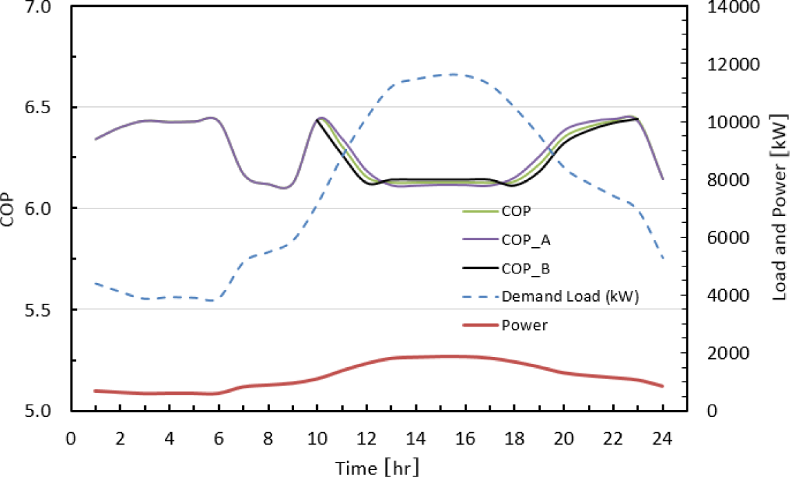
A typical cooling load of local tropical climate is applied to the CCS for both scenarios (I & II) in order to calculate the daily energy consumption by the CCS. The simulation results of the system’s COP, compression power and cooling load are shown in Figure 6 and Figure 7, for both scenarios respectively (partial & equal).
COP, chiller power and cooling load over 24 hours when chillers are operated on equal-loads (scenario-I)
COP, chiller power and cooling load over 24 hours, when chiller A is operated on full load and chiller B on part load (scenario-II)
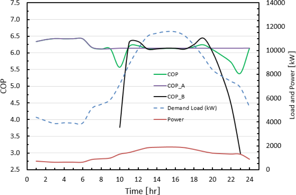
The system’s average-COP in the equally loaded (scenario-I) system is higher than the fully loaded (scenario-II), which results in lower power consumption while satisfying the same given cooling load. Therefore, in scenario-II where one chiller is operated at low PLR, the system’s average-COP is less and results in higher power consumption while meeting the same given cooling load.
The system’s COP reaches the maximum at 95% of the full load in the equal load (scenario-I), and exactly at the full load in the fully loaded (scenario-II). The illustration of this is revealed by the fact that the two chillers could not have identical optimal operating conditions. On the other hand, the minimum system’s COP in both scenarios (I & II) happens at the peak demand load as shown in Figures 6 and 7. The reason for this low COP is due to of the high Dry-Bulb Temperature (DBT) in this time of day, afternoon as demonstrated in Figure 8.
The results found in scenarios (I & II) are utilized in scenario-III (TES integration) by operating the CCS plant, both chillers, on the ultimate COP conditions in order to have the minimum energy consumption of the system.
The optimization framework that determines the optimal schedule scheme of the integrated CCS-TES system assumes a predicted COP as a function of the ambient Wet-Bulb Temperature (WBT). The optimal solution is represented by the loading schedule of both chillers, as well as, the charging and discharging of the TES tank along the optimization horizon (24 hours) as shown in Figure 9.
Determined chillers COP along the 24 hours
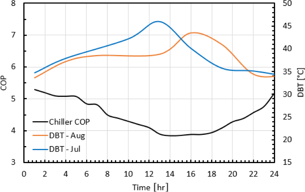
The optimization reveals that the two chillers tend to operate on full time during the first and last hours of the day because both of them have better COP at these timings. During the periods where only one chiller is required to run, such as between 12-19 h, the chiller B is operated since it has higher COP than chiller A at this particular period.
Preliminary results of the TES-chiller schedule optimization
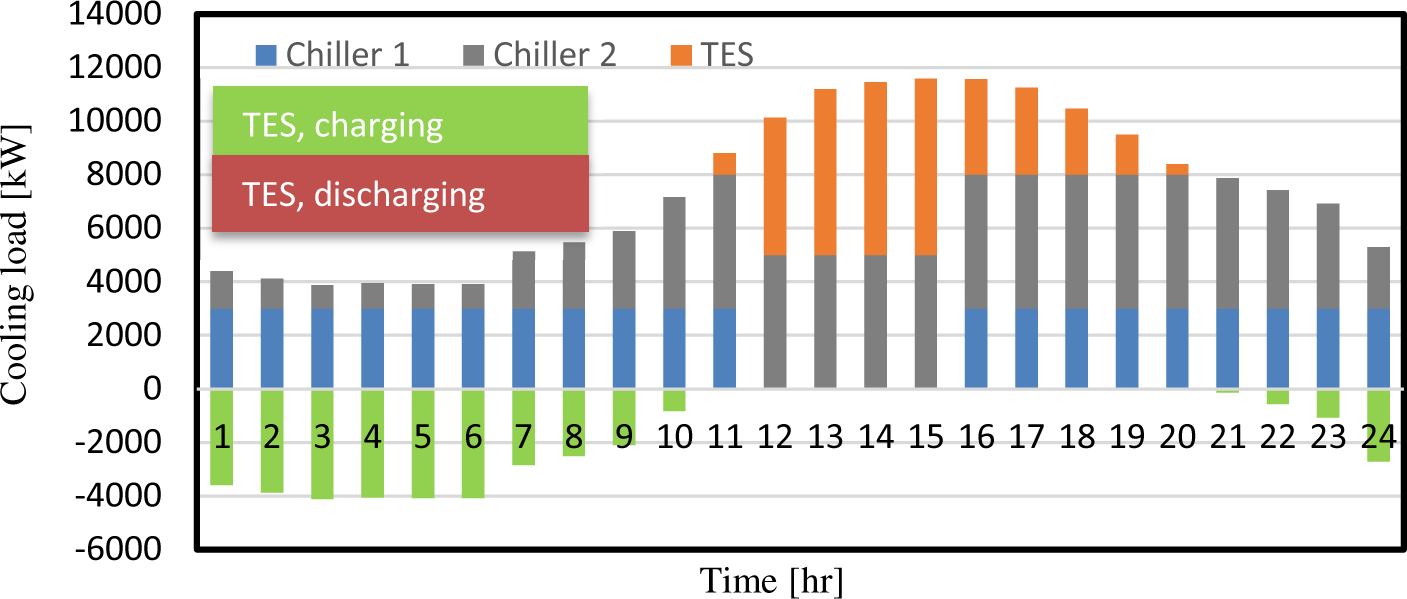
At 11.00 h, where the COP of the two chillers is lower as shown in Figure 8, the system starts to discharge the TES tank to meet the cooling demand while operating the two chillers at partial load. At 12.00 h, the chiller with a lower COP (chiller A) is set to off and both chiller B and the TES tank are expected to meet the cooling load demand. This situation takes place for four hours until the TES tank is relatively insufficient, at which case chiller A will be set to on again and the cycle repeats again.
The volume and surface area for the proposed cylindrical storage tank is 3,620 m3 and 1,306 m2, respectively. These specifications will result in losses of approximately 2,645 kWh, however, this value is subject to change depending on the insulation material of the TES tank.
It is worthy to notice that both chillers A and B have not exceeded 3,000 and 5,000 kW loadings respectively, which are significantly below their corresponding maximum capacities. This implies that there is a high potential to lower the capital cost of the CCS.
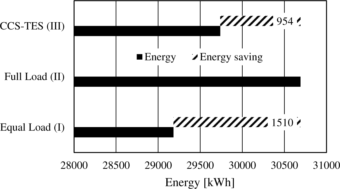
To summarize, the energy comparison for the three scenarios while satisfying the same demand is shown in Figure 10. Scenarios-I and -II are for CCS equal load and full load strategies, respectively. Scenario-III is for the CCS-TES integrated system. It can be clearly seen that the energy saving is the highest for scenario-I, however, the load must be equally divided between two chillers. On the other hand, scenario-III energy saving is less than scenario-I, however, it does not need two chillers. In addition, scenario-III energy saving can be improved by improving the TES tank design and/or its insulation material.
Energy comparison for the three scenarios
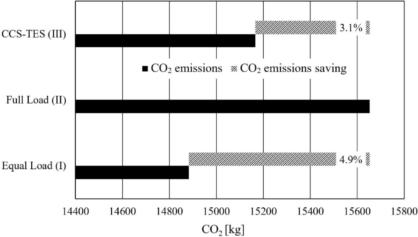
Carbon dioxide (CO2) emissions are estimated for each scenario using the 0.51 kg CO2/kWh emission factor for electricity production in the UAE [21] as shown in Figure 11. In the base scenario, CO2 emission is 15,653 kg CO2. Scenario-I has 4.9% less CO2 emissions and scenario-III has 3.1% less CO2 emissions.
CO2 emissions and saving of the three simulated scenarios
This paper investigated the potential benefits of integrating a thermal energy storage with a chiller cooling system as well as implemented optimal operation control between two chillers in parallel operation. Three scenarios were considered: I- conventional; two chillers cooling system with equal load, II- conventional; two chillers cooling system with one chiller on full load and the other chiller on partial load, III- conventional; two chillers cooling system with a thermal storage tank (chilled water). The two chillers are installed in Abu Dhabi, under hot and humid weather conditions, and therefore, the algorithm is developed for cooling load-based control. The chillers loading problem is not a straightforward task since every control response to any load variation would have a significant impact on the total system energy consumption.
The energy comparison between the considered scenarios showed that implementing two chillers with the equal load will save around 5% of the energy consumption and a corresponding percentage of CO2 emissions, however, it needs two chillers which may increase both initial and capital costs, whereas, the implementation of TES into the base CCS will save about 3% of the total energy consumption and a corresponding percentage of CO2 emissions. However, scenario-III has shaved about 30% of the peak load demand for 10 hours, giving the decision makers the option to eliminate more than 30% of the plant’s initial capacity that is designed to operate over 24-hours a day on a relatively constant load.
Moreover, the TES may improve the life cycle of the chillers since they are running relatively steadily regardless of the cooling load. In addition, it will reduce the initial and operation costs by reducing the chillers’ capacity and the number that are required to carry the cooling load. On the other hand, the exergy destruction resulting from continuously turning the chillers on and off will significantly drop.
Masdar city and Masdar Institute of Science and Technology support this study. This support is thankfully acknowledged.
| Cp | specific heat | [kJ/kgk] |
| DBT | dry bulb temperature | [°C] |
| Ρ | water density | [kg/m3] |
| TC | tank capacity | [kWh] |
| V | tank volume | [m3] |
| WBT | wet bulb temperature | [°C] |
| Q̇ | heat transfer rate | [kW] |
| Greek letters | ||
| ρ | density | [kg/m3] |
| ɛ | effectiveness | [-] |
| ΔT | temperature difference | [K] |
| Abbreviations | ||
| CCS | Chiller Cooling System | |
| CLC | Cooling Load Control | |
| COP | Coefficient of Performance | |
| PLR | Part Load Ratio | |
| TES | Thermal Energy Storage | |
| VFD | Variable Frequency Drive | |
- Statistical Report, 2016, http://www.adwec.ae/documents/report/2016/statistical%20report%201999-2016.pdf
- Environment Statistical Report, 2014, https://www.scad.ae/release%20documents/statistical%20yearbook_%202009.pdf
- ,
Amelioration of the Cooling Load Based Chiller Sequencing Control ,Appl. Energy , Vol. 168 ,pp 204-215 , 2016, https://doi.org/https://doi.org/10.1016/j.apenergy.2016.01.035 - ,
A New Solution for Loading Optimization of Multi-Chiller Systems by General Algebraic Modeling System ,Appl. Therm. Eng. , Vol. 84 ,pp 429-436 , 2015, https://doi.org/https://doi.org/10.1016/j.applthermaleng.2015.03.057 - ,
Modeling and Optimization of a Chiller Plant ,Energy , Vol. 73 ,pp 898-907 , 2014, https://doi.org/https://doi.org/10.1016/j.energy.2014.06.102 - ,
Optimal Chiller Loading for Energy Conservation Using a New Differential Cuckoo Search Approach ,Energy , Vol. 75 ,pp 237-243 , 2014, https://doi.org/https://doi.org/10.1016/j.energy.2014.07.060 - ,
An Innovative Approach for Demand Side Management-Optimal Chiller Loading by Simulated Annealing ,Energy , Vol. 31 (12),pp 1547-1560 , 2006, https://doi.org/https://doi.org/10.1016/j.energy.2005.10.018 - ,
Optimal Chilled Water Temperature Calculation of Multiple Chiller Systems Using Hopfield Neural Network for Saving Energy ,Energy , Vol. 34 (4),pp 448-456 , 2009, https://doi.org/https://doi.org/10.1016/j.energy.2008.12.010 - ,
Model-Based Optimization for Vapor Compression Refrigeration Cycle ,Energy , Vol. 55 ,pp 392-402 , 2013, https://doi.org/https://doi.org/10.1016/j.energy.2013.02.071 - ,
Thermoeconomic Optimization of Subcooled and Superheated Vapor Compression Refrigeration Cycle ,Energy , Vol. 31 (12),pp 1772-1792 , 2006, https://doi.org/https://doi.org/10.1016/j.energy.2005.10.015 - ,
Efficient Low-Lift Cooling with Radiant Distribution, Thermal Storage, and Variable-Speed Chiller Controls ‒ Part I: Component and Subsystem Models ,HVAC&R Res. , Vol. 15 (2),pp 366-400 , 2009, https://doi.org/https://doi.org/10.1080/10789669.2009.10390842 - , Model Predictive Control of Thermal Energy Storage in Building Cooling Systems, Proceedings of the 48th IEEE Conf. Decis. Control Held Jointly with 2009 28th Chinese Control Conf., 2009
- ,
Model Predictive Control of Central Chiller Plant with Thermal Energy Storage via Dynamic Programming and Mixed-Integer Linear Programming ,IEEE Trans. Control Syst. Technol. , Vol. 12 (2),pp 565-579 , 2015, https://doi.org/https://doi.org/10.1109/TASE.2014.2352280 - ,
Optimal Scheduling of Buildings with Energy Generation and Thermal Energy Storage Under Dynamic Electricity Pricing Using Mixed-Integer Nonlinear Programming ,Appl. Energy , Vol. 147 ,pp 49-58 , 2015, https://doi.org/https://doi.org/10.1016/j.apenergy.2015.02.060 - ,
Energy Efficient Control of HVAC Systems with Ice Cold Thermal Energy Storage ,J. Process Control , Vol. 24 (6),pp 773-781 , 2014, https://doi.org/https://doi.org/10.1016/j.jprocont.2014.01.008 - ,
Role of PCM Addition on Stratification Behavior in a Thermal Storage Tank – An Experimental Study ,Energy , Vol. 115 (Part 1),pp 1168-1178 , 2016, https://doi.org/https://doi.org/10.1016/j.energy.2016.09.014 - ,
A Simplified Model to Study the Location Impact of Latent Thermal Energy Storage in Building Cooling Heating and Power System ,Energy , Vol. 114 ,pp 885-894 , 2016, https://doi.org/https://doi.org/10.1016/j.energy.2016.08.062 - ,
The Role of Cool Thermal Energy Storage (CTES) in the Integration of Renewable Energy Sources (RES) and Peak Load Reduction ,Energy , Vol. 48 (1),pp 108-117 , 2012, https://doi.org/https://doi.org/10.1016/j.energy.2012.06.070 - , , Principles of Heating, Ventilation and Air Conditioning in Buildings, 2013
- , General Algebraic Modeling System (GAMS) Release 24.2.1, 2013
- , https://www.ead.ae/documents/PDF-files/AD-greenhouse-gas-inventory-eng.pdf