


Energy accounts for over 70% of total Greenhouse Gas (GHG) emissions [1], and the share of energy-related GHG emissions caused by cities have been estimated to account for over 70% [2]. This highlights the mitigating role of cities in energy-related GHG emissions and climate change in general. In favor of this, it has been shown that cities are efficient in promoting national energy policies (e.g. [3], [4]).
Utilization of waste heat has a powerful potential to reduce GHG emissions globally [5]. The original idea of the District Heating (DH) system is that heat can be recycled from sources where it would otherwise be wasted [6]. For instance, in the Nordic countries, where DH has a long tradition and the total supply of DH is 130 TWh/year [7], [8], heat for the DH network is produced in centralized heating plants, such as Combined Heat and Power (CHP) plants, which in most cases is a versatile fuel mix.
Despite high figures for the amount of CHP in DH systems, the amount of industrial waste heat used as a heat source in DH systems is still low, even though it is regarded as a vital means of increasing energy efficiency. In the new heat roadmap for Europe, Connolly et al. [9] mapped the yearly potential of industrial excess heat in DH networks in the EU27 countries for 2,710 PJ, which is almost twice as much as the total DH in 2010. The amount of industrial excess heat used in DH networks accounted for only 0.9% of the mapped potential in the year 2010 [9]. In Sweden, the amount of industrial waste heat used in DH systems was the highest out of all these countries in 2011 ‒ it accounted for 7% (3,852 GWh) of the total fuel input [10]. The potential of industrial waste heat utilization is also studied in China [11], Spain [12], and Croatia [13]. Although the potential of industrial waste heat is shown to be significant, the actual GHG impacts are unclear when heat pumps are needed to increase the temperature of utilized waste heat to be suitable for DH network. Although waste heat as itself can be GHG emission free, energy used to increase and distribute the heat may not be. Thus, assessment of the GHG emission implications is needed in order to understand actual GHG emissions. However, assessment of such implications is relatively complex.
For GHG assessment, three different scopes have been suggested by the GHG Protocol Corporate Standard [14]. Scope 1 emissions are direct GHG emissions from sources within the city boundary. Scope 2 expands the definition by including GHG emissions occurring as a consequence of the grid supplied electricity, heat, steam, and/or cooling within the city boundaries. Scope 3 further expands the definition by including all the other GHG emissions outside the city boundaries caused by activities within the city boundaries. For stationary energy-related assessments, the difference between Scope 2 and Scope 3 is that Scope 3 also includes indirect GHG emissions from the use of energy. Scopes 1-3 together form the carbon footprint of the studied object, e.g. an individual, a city, or a nation ‒ following the definition of Wiedmann and Minx [15].
In addition to indirect emissions, consequential implications also occurred from the actions needed to be recognized in order to have a comprehensive understanding. Life Cycle Assessment (LCA) is a method capable of accounting for the global impact of activities taking place in a certain geographic region. From the perspective of how global implications are accounted for, there are two approaches for LCA ‒ Attributional and Consequential LCA (ALCA & CLCA). The first only accounts for the emissions through the production and delivery chains, whereas the latter tries to capture the related change in the system in general, following a change in one component. These two approaches can thus lead to completely different perceptions of the matter and ALCA, thus misleading policy makers [16]. Especially in the electricity grid, the CLCA approach increases the GHG implications [17] and has also emphasized effects on cities’ carbon footprints [18].
For a city-level assessment of energy-related impacts, although often needed to understand the actual implications, the CLCA approach complicates the assessment of impacts and the decision-making regarding energy choices [19]. Energy systems, the utilization of energy sources, and relevant matters need to be assessed based on consequential impacts as well when the assessment is based on the CLCA approach. Within energy system studies, consequential system impacts are well-studied and often referred to as marginal system impacts [20]. Marginal energy impacts are changes made to an energy production system and production portfolio. Marginal production technology is usually the most expensive and most harmful to the environment. This potentially improves the efficiency made through limiting energy demand, but it increases the relevance of consequential implications occurred from the increase in energy demand.
Despite the broad existing research in the areas of assessment methods and waste heat utilization, the actual GHG emission implications from waste heat utilization and from the ALCA and CLCA perspectives within different scopes is a relatively untouched area. Such implications are important to understand when reaching negative GHG emission implications within municipal and national boundaries. Understanding of consequential implications when waste heat replaces alternative energy source but utilize other is beneficial when identifying the conditions in which negative GHG emission implications are evident. Additionally, understanding of consequential implications is important when deciding where to place waste heat sources.
This case study assesses a case where a data center is located in a city and its waste heat is utilized within the municipal DH system, replacing natural gas as a heat source. The case has been previously assessed from the technical and economic perspectives, and it was proposed that CLCA would be an appropriate approach for GHG implication assessment [21]. The case study assesses GHG emission implications within GHG Protocol’s Scopes 1-3, as proposed in the previous case study. The CLCA perspective is included and considered within Scope 3 assessments. The purpose is to illustrate how utilization of waste heat to decrease municipal-bounded GHG emissions can lead to an increase in GHG emissions within wider boundaries.
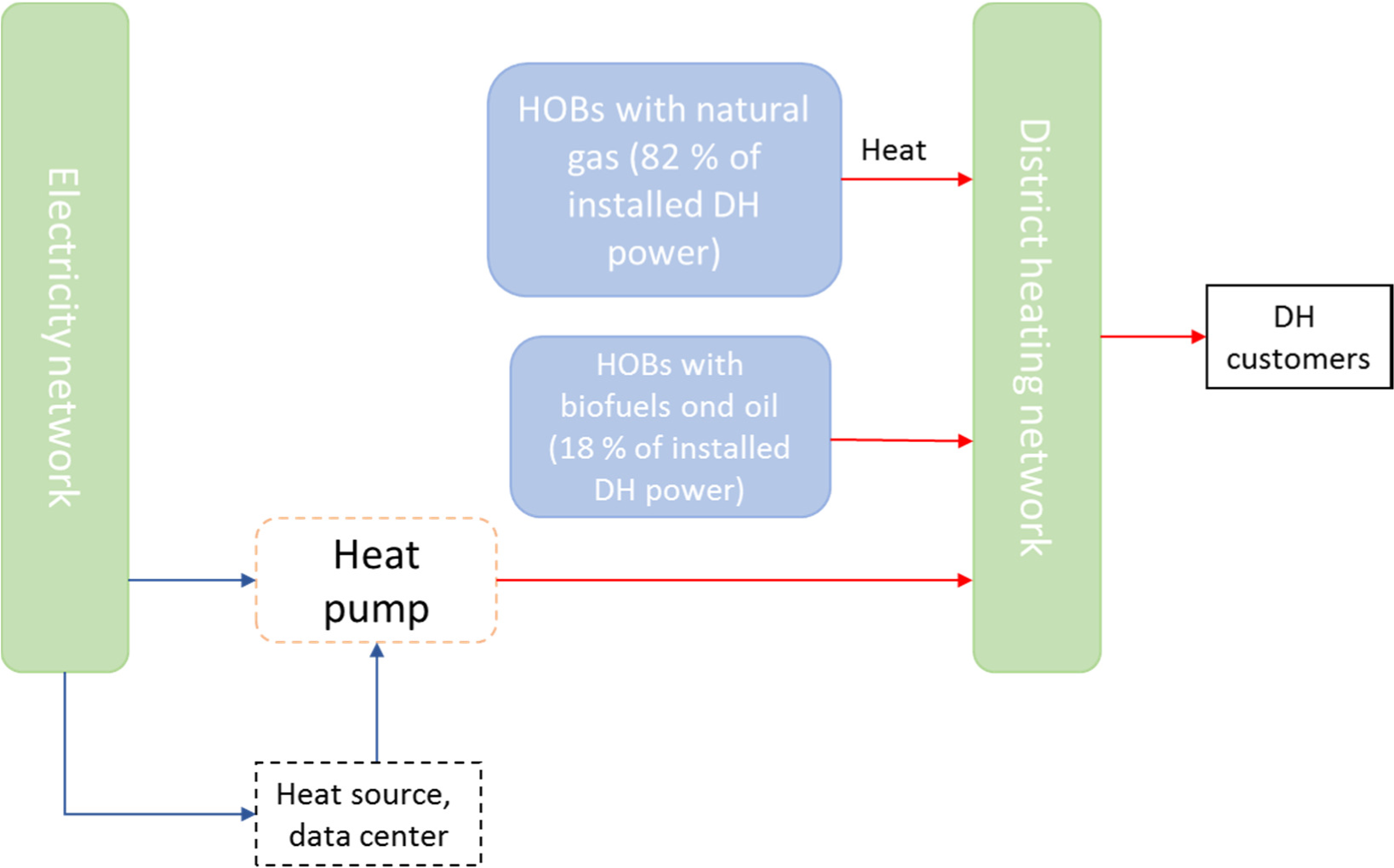
Mäntsälä is a small city with 20,853 inhabitants (2016) located in southern Finland. The city of Mäntsälä owns the company Nivos Energia Oy, which itself owns a DH network. DH production is covered with Heat-Only Boilers (HOB) located along the city, where natural gas plays a major role, as shown in Figure 1 and Table 1. A major new electricity consumption unit was added in 2016 when a data center was built. The site and detailed spatial location were chosen so that it was technically feasible to utilize the waste heat in a municipal energy system and DH network.
DH network production in Mäntsälä
Information of DH network in Mäntsälä 2016 [22]
| DH production specifications | |
| Number of HOBs | 11 |
| Length of the heating network [km] | 37.2 |
| Number of consumer points | 210 |
| Customer contract power total | 38.1 |
| Net production [GWh] | 54.4 |
| Heat supply [GWh] | 54.4 |
| Heat consumption [GWh] | 44.0 |
| Heat delivery and losses [GWh] | 10.4 |
| Boiler conversion losses [%] | 10 |
| Fuels | |
| Light oil [GWh] | 2.8 |
| Natural gas [GWh] | 30.5 |
| Bio fuels [GWh] | 8.7 |
| Heat pump supply [GWh] | 16.1 |
| Light oil [CO2eq/kWh] | 261.7 |
| Natural gas [CO2eq/kWh] | 198.1 |
| Bio fuels [CO2eq/kWh] | 0 |
The assessment methods employed in the study are based on ALCA and CLCA as well as direct GHG emission assessment. Assessment boundaries are GHG Protocol’s Scopes 1-3 where ALCA and CLCA is performed within their scope. For Scopes 1 and 2, only direct emissions are considered. The Scope 1 boundary definition used is a city’s own direct production emissions. For Scope 2, Scope 1 emissions are added by direct emissions from energy use that is produced outside the city boundaries. In this case, such emissions occurred from the electricity supplied from the grid. For Scope 3, the boundary is the national border and the Finnish grid with indirect emissions from energy production. For a consequential implication in CLCA, marginal electricity production is assumed to be national condensing power production with its average emissions calculated as presented in Table 2. The CLCA approach is limited to cover only instant marginal energy emission implications. Thus, wider consequential system implications are excluded.
Calculation definitions and principals
| Scope | LCA | Out-of-jurisdiction implications | GHG emission range’s minimum (L) or maximum (H) values [direct only (D)] | Calculation of energy-based emission implications | |
|---|---|---|---|---|---|
| Scope 1 emission implications | 1 | A | + | D | Cimp = –Eh × GHGng |
| Scope 2 emission implications | 2 | A | + | D | Cimp = –Eh × GHGng + Ep × GHGel + Ed × GHGel |
| Scope 2 emission implications excluding out-of-jurisdiction implications | 2 | A | - | D | Cimp = –Eh × GHGng + Ep × GHGel |
| Scope 3 emission implications (minimum values for emissions) | 3 | A | + | L | Cimp = –Eh × GHGngl + Ep × GHGell + Ed × GHGell |
| Scope 3 emission implications excluding out-of-jurisdiction implications (minimum values for emissions) | 3 | A | - | L | Cimp = –Eh × GHGngl + Ep × GHGell |
| Scope 3 emission implications (maximum values for emissions) | 3 | A | + | H | Cimp = –Eh × GHGngm + Ep × GHGelm + Ed × GHGelm |
| Scope 3 emission implications excluding out-of-jurisdiction implications (maximum values for emissions) | 3 | A | - | H | Cimp = –Eh × GHGngm + Ep × GHGelm |
| Scope 3 emission implications CLCA (minimum values for emissions) | 3 | C | + | L | Cimp = –Eh × GHGngl + Ep × GHGellmarg + Ed × GHGellmarg |
| Scope 3 emission implications CLCA excluding out-of-jurisdiction implications (minimum values for emissions) | 3 | C | - | L | Cimp = –Eh × GHGngl + Ep × GHGellmarg |
| Scope 3 emission implications CLCA (maximum values for emissions) | 3 | C | + | H | Cimp = –Eh × GHGngm + Ep × GHGelmmarg + Ed × GHGelmmarg |
| Scope 3 emission implications CLCA excluding out-of-jurisdiction implications (maximum values for emissions) | 3 | C | - | H | Cimp = –Eh × GHGngm + Ep × GHGelmmarg |
Cimp = GHG implications [t CO2]
Eh = Supplied heat energy from the heat pump unit [GWh]
GHGng = CO2eq of natural gas and boiler-based district heat [t CO2/GWh]
Ep = Electricity used by the heat pump [GWh]
GHGel = Direct CO2eq of electricity from the grid [t CO2/GWh]
Ed = Electricity used by the data center [GWh]
GHGngl = Direct + indirect CO2eq of natural gas and boiler-based district heat (lowest emission value from the range) [t CO2]
GHGell = Direct + indirect CO2eq of electricity (lowest emission value from the range) [t CO2/GWh]
GHGngm = Direct + indirect CO2eq of natural gas and boiler-based district heat (highest emission value from the range) [t CO2/GWh]
GHGelm = Direct + indirect CO2eq of electricity (highest emission value from the range) [t CO2/GWh]
GHGellmarg = Direct + indirect CO2eq of marginal electricity (lowest emission value from the range) [t CO2/GWh]
GHGelmmarg = Direct + indirect CO2eq of marginal electricity (maximum emission value from the range) [t CO2/GWh]
The assessments consider the emission implications rather than the complete emissions of the city. Implications are specified to cover implications from the integration of the data center as well as the utilization of the waste heat generated. Energy consumption units are the data center and the heat pump unit, which is owned by the municipal DH company. Waste heat replaces the natural gas-based boiler, and such emission mitigation implications are considered to be emission-negative.
Assessments in Scopes 2 and 3 also consider data center energy usage as an out-of-jurisdiction actor for the municipality, presenting only in-jurisdiction GHG emission implications as defined by GHG Protocol’s Policy and Action Standard [23], but including the heat pump’s electricity usage, as it is owned by the municipal energy company. The purpose of this is to compare results when it is assumed that the specific energy use would exist regardless.
For the supplied heat, direct GHG emission implications are calculated from the emissions from the production of the energy excluding network losses, which are considered to be equal. For electricity production and with ALCA and CLCA, network losses are also considered.
Eleven different assessments are performed with different boundaries and assessment methods. Table 2 presents assessment calculation definitions and principals.
The research study utilizes public and site-specific data sources for the GHG implication assessments. Site-specific energy measurements are used to measure actual energy inputs and outputs, and national energy statistics are used to calculate direct emissions from the use of energy. For the indirect energy emissions, a study by Cherubini et al. [24] is used to specify uncertainty ranges.
Site-specific energy measurements are based on real-time energy monitoring of the data center, the heat pump unit, and the municipal DH company from 2016. Both purchased electricity and supplied heat are monitored by the data center and reported monthly. The heat pump unit operated by the municipal DH company is reported accordingly. Table 3 presents the monthly energy input and output of the data center.
Energy input-output of the site under analysis
| Consumed electricity (heat pump) [MWh] | Supplied heat from the heat pump [MWh] | Supplied heat from the data center [MWh] | Coefficient of Performance | Consumed electricity (data center) [MWh] | |
|---|---|---|---|---|---|
| January 2016 | 331 | 1,042 | 663 | 3.2 | 3,411 |
| February 2016 | 326 | 1,016 | 807 | 3.1 | 3,335 |
| March 2016 | 387 | 1,167 | 593 | 3 | 3,730 |
| April 2016 | 521 | 1,624 | 470 | 3.1 | 3,746 |
| May 2016 | 284 | 851 | 586 | 3 | 4,019 |
| June 2016 | 245 | 746 | 576 | 3 | 3,820 |
| July 2016 | 248 | 752 | 476 | 3 | 4,034 |
| August 2016 | 408 | 1,341 | 927 | 3.3 | 4,277 |
| September 2016 | 470 | 1,552 | 1,176 | 3.3 | 4,183 |
| October 2016 | 627 | 2,060 | 1,333 | 3.3 | 4,380 |
| November 2016 | 621 | 2,063 | 1,420 | 3.3 | 4,363 |
| December 2016 | 641 | 2,124 | 663 | 3.3 | 4,784 |
Statistics Finland and the Finnish energy industry are compiling monthly electricity production of CO2 emissions based on the energy allocation method. Table 4 presents monthly electricity CO2 emissions within Finland. These values are used to calculate monthly direct emission implications occurring from the consumption of electricity when ALCA is performed. The relatively low emissions during the summer is due to decreased consumption and thus decreased production of higher emission production plants with higher marginal cost.
Monthly average emissions of purchased electricity from the national grid [25]
| CO2 emissions of average electricity [t CO2eq/GWh] | |
|---|---|
| January 2016 | 146 |
| February 2016 | 104 |
| March 2016 | 104 |
| April 2016 | 98 |
| May 2016 | 75 |
| June 2016 | 57 |
| July 2016 | 38 |
| August 2016 | 60 |
| September 2016 | 90 |
| October 2016 | 147 |
| November 2016 | 155 |
| December 2016 | 127 |
Table 5 presents monthly electricity production shares per production technology in 2016. These values are used to calculate monthly production emissions including indirect shares. Indirect emissions and emission ranges are calculated by multiplying these values with the emission ranges presented in Table 6. For thermal power production, fuel sources are presented in Table 7. For the peat emission range’s lowest value, 1,150 kg CO2eq/MWh was used, as presented by Style and Jones [26]. For the highest value, a factor between coal-based electricity production’s lowest and highest values were used, giving 1,920 kg CO2eq/MWh for the peat power production’s highest value. 70 to 85 kg CO2eq/MWh were used for emission ranges for local municipal DH, as presented in Cherubini et al. [24].
Monthly 2016 electricity production shares [25]
| January | February | March | April | May | June | July | August | September | October | November | December | ||
|---|---|---|---|---|---|---|---|---|---|---|---|---|---|
| Hydro power | [MWh] | 1,404 | 1,404 | 1,413 | 1,426 | 1,626 | 1,291 | 1,223 | 1,392 | 1,361 | 1,128 | 942 | 1,024 |
| Wind power | 221 | 235 | 216 | 198 | 150 | 201 | 144 | 292 | 237 | 250 | 407 | 516 | |
| Solar power | - | - | - | - | - | - | - | - | - | - | - | - | |
| Nuclear power | 2,064 | 1,928 | 2,061 | 1,840 | 1,503 | 1,692 | 1,987 | 1,702 | 1,606 | 1,950 | 1,985 | 1,961 | |
| Conv. thermal power | 3,385 | 2,582 | 2,593 | 2,118 | 1,492 | 1,204 | 1,077 | 1,204 | 1,337 | 2,331 | 3,016 | 2,847 | |
| Co-generation | 2,862 | 2,307 | 2,287 | 1,811 | 1,232 | 1,016 | 928 | 928 | 976 | 1,702 | 2,386 | 2,431 | |
| District heating | 1,913 | 1,478 | 1,411 | 1,055 | 533 | 368 | 238 | 238 | 422 | 1,048 | 1,632 | 1,651 | |
| Industry | 949 | 829 | 875 | 756 | 699 | 648 | 690 | 690 | 554 | 654 | 754 | 781 | |
| Condense | 523 | 275 | 307 | 306 | 260 | 188 | 149 | 276 | 361 | 628 | 630 | 416 | |
| Conventional | 521 | 275 | 306 | 305 | 258 | 188 | 147 | 275 | 361 | 628 | 629 | 416 | |
| Gasturbine, etc. | 2 | 0 | 1 | 1 | 2 | 0 | 2 | 1 | 0 | 0 | 0 | 0 | |
| Production total | 7,073 | 6,149 | 6,283 | 5,581 | 4,772 | 4,389 | 4,431 | 4,590 | 4,542 | 5,659 | 6,349 | 6,349 |
Emission ranges for energy production including indirect emissions [24]
| Lowest values | Highest values | |
|---|---|---|
| [t CO2eq/GWh] | ||
| Biomass | 54 | 108 |
| Wind | 4 | 36 |
| Hydro | 2 | 36 |
| Solar | 54 | 144 |
| Coal | 1,080 | 1,800 |
| Oil | 720 | 1,080 |
| Nuclear | 18 | 108 |
| Natural gas | 360 | 720 |
Thermal power production fuel sources in 2016 [27]
| Electricity [GWh] | |
|---|---|
| Condensing production | |
| Oil | 66 |
| Coal | 2,084 |
| Natural gas | 25 |
| Other fossil-based | 508 |
| Peat | 448 |
| Wood industry’s waste liquors | 338 |
| Other wood sources | 708 |
| Other renewables | 90 |
| Other sources | 51 |
| Total | 4,319 |
| Cogeneration | |
| Oil | 103 |
| Coal | 4,468 |
| Natural gas | 3,617 |
| Other fossil based | 405 |
| Peat | 2,284 |
| wood industry’s waste liquors | 5,031 |
| Other wood sources | 4,105 |
| Other renewables | 577 |
| Other sources | 291 |
| Total | 20,880 |
This section presents the results within the reference year of 2016. Additionally, this section presents the results when it is assumed that half of the waste heat would be utilized, as it is the purpose of the further site development.
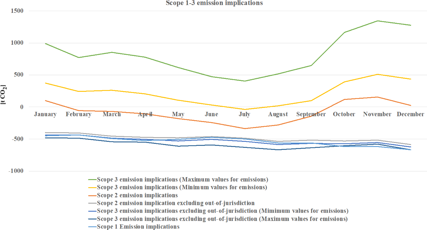
Figure 2 presents monthly-based assessment results of the reference year within Scopes 1-3. Seven different scope and assumption setups are included: Scope 1 implications, Scope 2 implications, including and excluding an out-of-jurisdiction actor, and Scope 3 implications, including and excluding an out-of-jurisdiction actor and with the minimum and maximum range in energy emission. It is shown that Scope 1 together with Scopes 2 and 3 when out-of-jurisdiction is excluded have a similar amount of negative GHG emission implications. When Scopes 2 and 3 are assessed with in-jurisdiction implications, the results show GHG emission positive implications. Scope 2 with in-jurisdiction implications shows the lowest GHG emission implications of these, reaching negative implications in July and August. Scope 3 with a minimum range of values for energy emissions shows the second highest implications, and a similar same scope with maximum range values for energy emissions shows the highest.
Scopes 1-3 emission implications in 2016 (the second Scope 2 assessment excludes data center electricity usage as an out-of-jurisdiction actor, Scope 3 assessments consider indirect emissions and emission uncertainty ranges as well, although the energy system’s performance is closer to the lowest values)
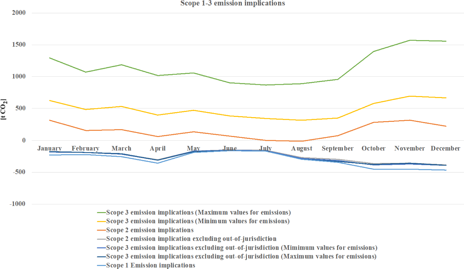
Figure 3 presents Scope 3 assessment results with CLCA and the condensing power production marginal energy perspective. Four different assumption setups are assessed ‒ Scope 3 including and excluding out-of-jurisdiction implications and with minimum and maximum range values for energy emissions. The results show that all the assumption setups show positive GHG emission implications. When excluding out-of-jurisdiction, assessments shows relatively low implications. The reason why the Scope 3 emission implications excluding out-of-jurisdiction implications show lower emission implications with maximum values is due to the relatively big decrease in locally used natural gas in relation to the increased consumption of electricity, both with higher GHG emission values. When out-of-jurisdiction is included, GHG emission implications are significant.
Consequential life-cycle assessment implications in 2016, where a condensing production fuel mix is considered to act as marginal energy production. Two assessments consider data center electricity as an out-of-jurisdiction actor
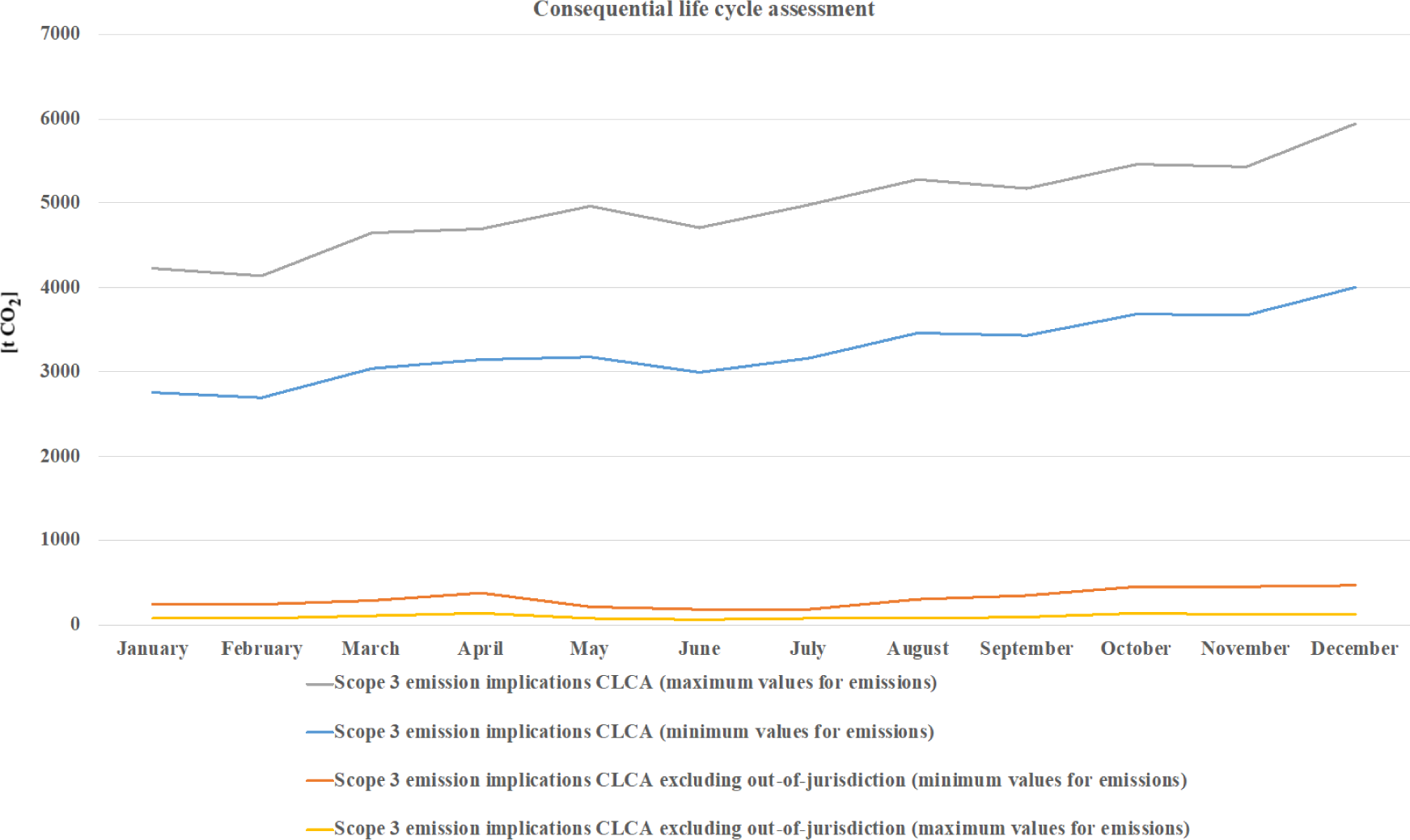
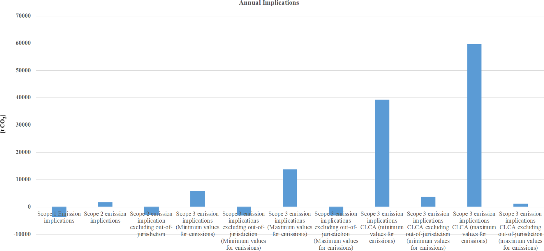
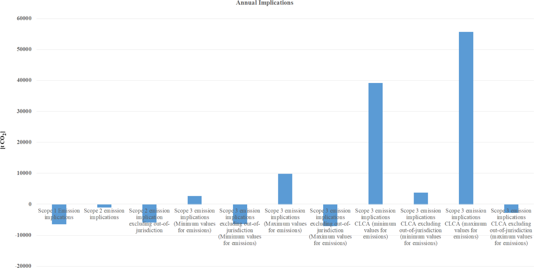
Figure 4 presents annual GHG emission implications cumulatively. It is seen that the wider the boundary within the assessment is, the higher the GHG emission implications are when out-of-jurisdiction implications are included.
Annual implications within all assessments and scopes [from left to right: Scope 1 emission implications, Scope 2 emission implications, Scope 2 emission implications excluding out-of-jurisdiction, Scope 3 emission implications (minimum values for emissions), Scope 3 emission implications excluding out-of-jurisdiction (minimum values for emissions), Scope 3 emission implications (maximum values for emissions), Scope 3 emission implications excluding out-of-jurisdiction (maximum values for emissions), Scope 3 emission implications CLCA (minimum values for emissions), Scope 3 emission implications CLCA excluding out-of-jurisdiction (minimum values for emissions), Scope 3 emission implications CLCA (maximum values for emissions), and Scope 3 emission implications CLCA excluding out-of-jurisdiction (maximum values for emissions)]
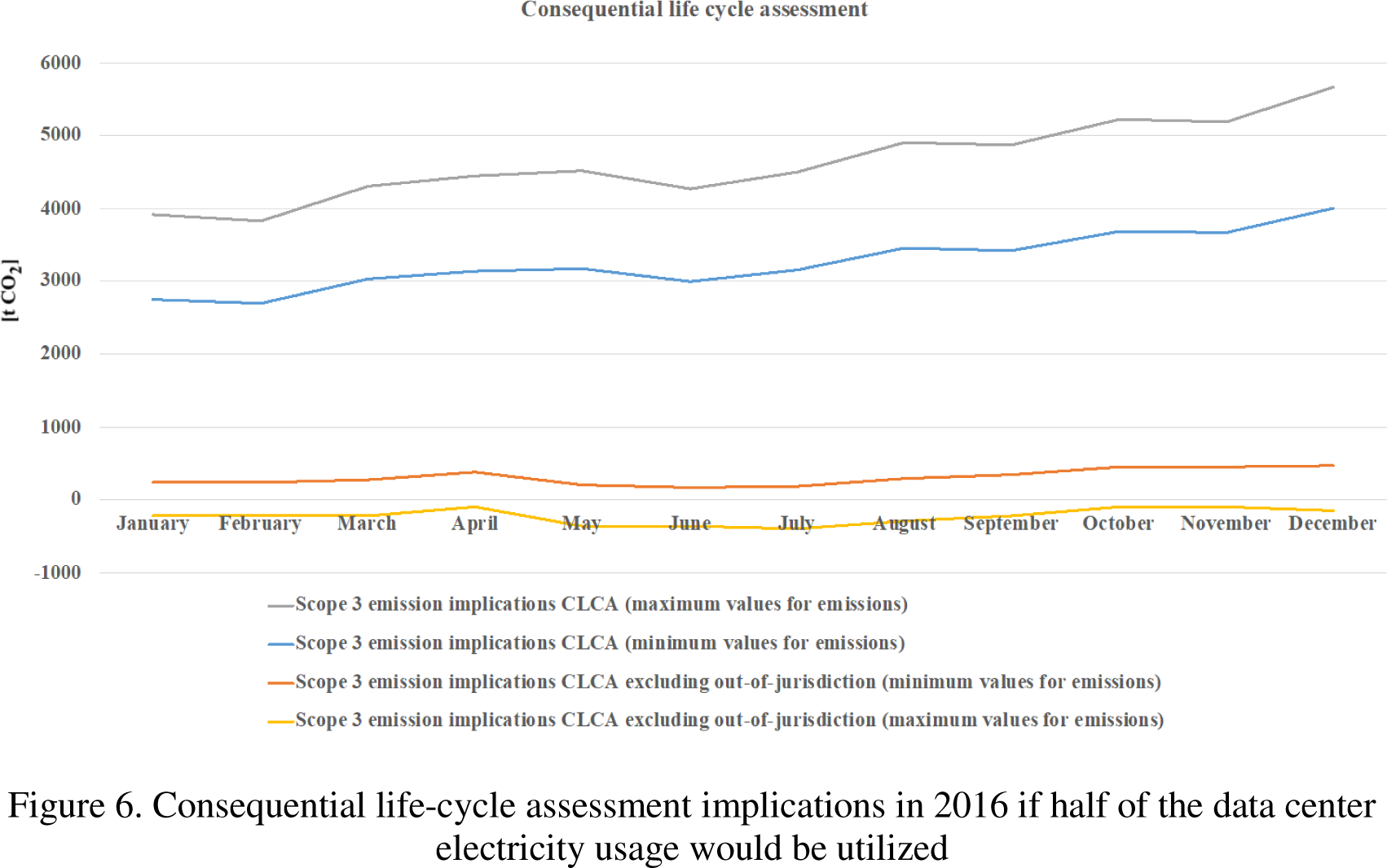
As the development plan of the site is to utilize half of the data center’s electricity consumption as waste heat, it is relevant to perform such a sensitivity analysis. Figures 5-7 present the results according to previous figures and assumptions. Updated results show significant differences. Previously with ALCA-based assessments, only Scope 1 together with Scopes 2 and 3 excluding out-of-jurisdiction implications showed negative GHG emission implications. Now also Scope 2 GHG emission implications are negative, and a significant reduction is shown for every scope and assumption setup. GHG emission reduction for CLCA-based assessments are shown as well in Figure 6 and Figure 7. Now also the CLCA-based Scope 3 assessment with maximum range values for energy and out-of-jurisdiction assumptions is seen to have negative GHG emission implications.
Scopes 1-3 assessment implications in 2016 if half of the data center electricity usage would be utilized according to the development plans
Consequential life-cycle assessment implications in 2016 if half of the data center electricity usage would be utilized
Annual implication within all the assessments and scopes when half of the data center electricity usage is utilized [from left to right: Scope 1 emission implications, Scope 2 emission implications, Scope 2 emission implications excluding out-of-jurisdiction, Scope 3 emission implications (minimum values for emissions), Scope 3 emission implications excluding out-of-jurisdiction (minimum values for emissions), Scope 3 emission implications (maximum values for emissions), Scope 3 emission implications excluding out-of-jurisdiction (maximum values for emissions), Scope 3 emission implications CLCA (minimum values for emissions), Scope 3 emission implications CLCA excluding out-of-jurisdiction (minimum values for emissions), Scope 3 emission implications CLCA (maximum values for emissions), and Scope 3 emission implications CLCA excluding out-of-jurisdiction (maximum values for emissions)]
The results demonstrated how utilization of waste heat to reduce municipal boundary GHG emissions can increase GHG emissions within wider boundaries. The results showed that the potential for decreasing GHG emissions as presented in studies such as [9], [13] are generalized, and actual GHG emission implications are complex to assess and may even lead to GHG emission growth.
As presented in studies such as [14]-[18], the results showed that the choice of assessment method and boundaries greatly affects GHG emission and emission implication results. The assessment method can even determine whether the implications are positive or negative. For municipalities, it is easy to use Scope 1 emissions and only direct emissions, as it often also accounts for the lowest emissions. However, as recommended by the GHG Protocol [24], for a more comprehensive assessment, a wider boundary needs to be used instead. This is important, as it would otherwise be relatively easy to outsource the GHG emissions. The results showed that the amount of negative emission implications shown in Scope 1 can be many times greater and positive in Scope 3.
The results also showed the importance of energy systems’ marginal system implications in municipal decision making and municipal GHG emission implication contexts. The results followed previous research findings that the choice between ALCA and CLCA can lead to completely different perceptions on the matter. With the ALCA method, all the assessment results were within a relatively normal range. From the CLCA perspective, on the other hand, the results showed a significant increase in GHG emissions when out-of-jurisdiction was included.
Results also showed that when including indirect energy emission ranges to the ALCA and CLCA perspectives, the complexity even increases. This makes it hard for municipal actors to assess actual GHG emission implications.
Although the assessments were targeted to cover a significant share of assessment scopes and assumptions, numerous uncertainties still exist. Firstly, energy emission ranges were utilized covering practically all the actual production methods. One can make a site comparison between the highest ranges and between the lowest ranges, as actual alternative production methods may vary between. Secondly, a reference year was assessed instead of the lifetime of the site. As energy systems are developing, these assessment results change accordingly. Thirdly, a scenario where the data center would not be integrated was not performed. As the results were implications, this would have been important to understand especially if a lifetime assessment would have been performed.
From the national boundary point of view, the data center as an out-of-jurisdiction actor is an important matter when mitigating GHG emissions. If that actor and its electricity consumption would exist in any case somewhere within the national boundary, the question would be where to best place it and where would its waste heat generate the most GHG emission mitigation. For this purpose, the results show that the location is relatively good, even from the CLCA perspective, as the condensing power generation fuel mix would not necessarily play such a major role as a marginal production, especially when assessing within a lifetime. From the global GHG emission mitigation perspective, it is important to recognize other possible locations, which energy sources are available in those locations, and the possibility to utilize waste heat.
For extensive GHG emission impact management within different scopes, it is proposed that a municipal actor should focus on Scopes 2 and 3 GHG emission implications from the ALCA and CLCA perspectives in addition to initial Scope 1 emissions. The aim should not be to minimize Scope 1 emissions, but to identify methods to minimize Scope 1 emissions as well as Scope 2 and 3 emissions as well.
Although assessment covers different scopes with different assessment methods, there are still uncertainties that could further change the results. A major uncertainty is related to the limited CLCA used within the study. There are several possible consequences that could drastically change the outlook. First, if waste heat were not utilized, there would probably be other investments to be made to reduce local GHG emissions. Secondly, the assessment is done only for the reference year rather than the life cycle of the site. This means that development of different systems and actors are excluded, which is crucial when assessing the actual consequential implications. Thirdly, consequential implications of non-GHG emissions and larger boundary are excluded.
The case study’s purpose was to show that the utilization of waste heat to decrease municipal boundary GHG emissions may increase such emissions within wider boundaries. The case study assessed Greenhouse Gas Protocol’s Scopes 1-3 when waste heat generated by a data center was utilized within a municipal DH system, replacing natural gas-based heat. Although Scope 1 GHG emissions were shown to decrease, both Scope 2 and 3 GHG emissions were increased. Further development of waste heat utilization could recover half of the generated waste heat, which is enough to turn Scope 2 emissions negative. In order for negative GHG emissions within Scope 3, the location’s replaceable municipal DH GHG emissions would need to be higher, such as emissions from coal with poor energy efficiency. When assessing consequential and initial electricity system impacts within Scope 3, additional electricity production changes are needed in order to realize negative GHG emission implications.
We thank Tekes ‒ the Finnish Funding Agency for Innovation (Project 3000/31/15) ‒ and Marjatta and Eino Kollin Säätiö (Grant 1102) for enabling the study. Jani Laine conducted the research assessment, created the research design, and participated in all stages of preparing the manuscript. Kaisa Kontu conducted the energy research positioning and participated in all stages of preparing the manuscript. Jukka Heinonen and Seppo Junnila participated in the research framing and participated in all stages of preparing the manuscript.
- ,
Climate Watch , https://www.climatewatchdata.org - ,
World Energy Outlook 2008 , 2008 - ,
Centralisation and Decentralisation in Strategic Municipal Energy Planning in Denmark ,Energy Policy , Vol. 39 (3),pp 1338-1351 , 2011, https://doi.org/https://doi.org/10.1016/j.enpol.2010.12.006 - ,
Municipal Energy-Planning and Development of Local Energy-Systems ,Applied Energy , Vol. 76 (1-3),pp 179-187 , 2003, https://doi.org/https://doi.org/10.1016/S0306-2619(03)00062-X - ,
Quantification of Global Waste Heat and its Environmental Effects ,Applied Energy , Vol. 235 ,pp 1314-1334 , 2019, https://doi.org/https://doi.org/10.1016/j.apenergy.2018.10.102 - ,
District Heating and Cooling ,Encyclopedia of Energy ,pp 841-848 , 2004, https://doi.org/https://doi.org/10.1016/B0-12-176480-X/00214-X - ,
Towards a Sustainable Nordic Energy System , 2010http://www.nordicenergy.org/wp-content/uploads/2012/02/Towards-a-Sustainable-Nordic-Energy-System.pdf - ,
Swedish District Heating—A System in Stagnation: Current and Future Trends in the District Heating Sector ,Energy Policy , Vol. 48 ,pp 449-459 , 2012, https://doi.org/https://doi.org/10.1016/j.enpol.2012.05.047 - ,
Heat Roadmap Europe: Combining District Heating with Heat Savings to Decarbonise the EU Energy System ,Energy Policy , Vol. 65 ,pp 475-489 , 2014, https://doi.org/https://doi.org/10.1016/j.enpol.2013.10.035 - ,
Large Heat Pumps in Swedish District Heating Systems ,Renewable and Sustainable Energy Reviews , Vol. 79 ,pp 1275-1284 , 2017, https://doi.org/https://doi.org/10.1016/j.rser.2017.05.135 - ,
Capturing the Invisible Resource: Analysis of Waste Heat Potential in Chinese Industry ,Applied Energy , Vol. 161 ,pp 497-511 , 2016, https://doi.org/https://doi.org/10.1016/j.apenergy.2015.10.060 - ,
Methodologies to Estimate Industrial Waste Heat Potential by Transferring Key Figures: A Case Study for Spain ,Applied Energy , Vol. 169 ,pp 866-873 , 2106, https://doi.org/https://doi.org/10.1016/j.apenergy.2016.02.089 - ,
Potential of Waste Heat in Croatian Industrial Sector ,Thermal Science , Vol. 16 (3),pp 747-758 , 2012, https://doi.org/https://doi.org/10.2298/TSCI120124123B - ,
, 2014http://ghgprotocol.org/sites/default/files/ghgp/standards/GHGP_GPC_0.pdf - ,
A Definition of ‘Carbon Footprint ,Ecological Economics Research Trends , Vol. 1 ,pp 1-11 , 2008 - ,
Using Attributional Life Cycle Assessment to Estimate Climate-Change Mitigation Benefits Misleads Policy Makers ,J. Industrial Ecology , Vol. 18 (1),pp 73-83 , 2013, https://doi.org/https://doi.org/10.1111/jiec.12074 - ,
The Complexity and Challenges of Determining GHG (Greenhouse Gas) Emissions from Grid Electricity Consumption and Conservation in LCA (Life Cycle Assessment): A Methodological Review ,Energy , Vol. 36 (12),pp 6705-6713 , 2011, https://doi.org/https://doi.org/10.1016/j.energy.2011.10.028 - ,
Consequential Implications of Municipal Energy System on City Carbon Footprints ,Sustainability , Vol. 9 (10),pp 1801 , 2017, https://doi.org/https://doi.org/10.3390/su9101801 - ,
Planning for a Low Carbon Future? Comparing Heat Pumps and Cogeneration as the Energy System Options for a New Residential Area ,Energies , Vol. 8 (9),pp 9137-9154 , 2015, https://doi.org/https://doi.org/10.3390/en8099137 - ,
Determining Marginal Electricity for Near-Term Plug-In and Fuel Cell Vehicle Demands in California: Impacts on Vehicle Greenhouse Gas Emissions ,J. of Power Sources , Vol. 195 (7),pp 2099-2109 , 2010, https://doi.org/https://doi.org/10.1016/j.jpowsour.2009.10.024 - ,
Future Views on Waste Heat Utilization: Case of Data Centers in Northern Europe ,Renewable and Sustainable Energy Reviews , Vol. 82 (2),pp 1749-1764 , 2018, https://doi.org/https://doi.org/10.1016/j.rser.2017.10.058 - ,
Statistics 2016 , https://energia.fi/en/ - ,
Policy and Action Standard – An Accounting and Reporting Standard for Estimating the Greenhouse Gas Effects of Policies and Actions , http://ghgprotocol.org/sites/default/files/standards/Policy%20and%20Action%20Standard.pdf - ,
Energy- and Greenhouse Gas-Based LCA of Biofuel and Bioenergy Systems: Key Issues, Ranges and Recommendations ,Resourc. Conserv. Recycl. , Vol. 53 (8),pp 434-447 , 2009, https://doi.org/https://doi.org/10.1016/j.resconrec.2009.03.013 - ,
Monthly Electricity Statistics 2016 , https://energia.fi/en/ - ,
Energy Crops in Ireland: Quantifying the Potential Life-Cycle Greenhouse Gas Reductions of Energy-Crop Electricity ,Biomass and Bioenergy , Vol. 31 (11),pp 759-772 , 2007, https://doi.org/https://doi.org/10.1016/j.biombioe.2007.05.003 - ,
Production of Electricity and Heat , 2016https://www.stat.fi/til/salatuo/2016/salatuo_2016_2017-11-02_tie_001_en.html