


Risk management, assessment, and mitigation for high-risk plants exposed to operational risks or natural hazards are built on: actions that attempt to identify potential risks [1]; data obtained from an accurate knowledge of territorial vulnerability [2]; monitoring network for assessing population exposure to pollution [3]; strategies aimed at supporting decisions on how to manage critical security issues [4] and how to select the appropriate response options for effective risk mitigation [5].
Even though many possible risks are foreseeable, one should always be prepared for unlikely scenarios that can lead to catastrophic failures. In this case, emergency response plans and forecast-based actions become strategic tools to deal with expected and unexpected variations of events.
In this context, most of the studies carried out until now are focused on: analyses devoted to identification and prioritisation of the risk; the development of tools to support proactive and reactive risk management [6]; or, after an event occurs and the situation is stable, how to perform a study on what occurred and how to determine the extent of damage [7]. Learning from past events is considered a suitable way to learn to handle an emergency [8]. However, this approach may not always be effective because a chain of events can manifest in ways different from what has already happened. What such an approach lacks is the availability of forecast models, capable for example of representing dry deposition phenomena through a new scheme of parameterization [9], to support emergency response activities involving the application of specialized atmospheric dispersion-modelling techniques [10] to track and predict the spread and deposition of hazardous substances [11].
To ensure high-quality modelling of air-pollution dispersion, it is necessary to focus on those variables of the meteorological description of the atmosphere that are vital for dispersion modelling. Nowadays various studies concerning the management of forecast data are available in the literature, from the classical approach of numerical validation [12] to the innovative approach of machine learning technique [13]. However, most of these models have a different purpose with respect to the application in emergency response such as, for example, geodetic applications [14] or production of dispersion maps to investigate past events [15].
For example, if those models can be used for a dispersion modelling system, their computational approach does not have temporal and spatial resolutions able to provide rapid response to emergency situations.
Furthermore, several models are based on local air quality monitoring stations for the prediction of air pollution and highlight limits due to accuracy problems relating to the available data sets [16]. Another critical aspect in forecasting the atmospheric dispersion is in fact associated with the meteorological data used, which represent one of the main sources of uncertainty [17].
Research was carried out at the Engineering Department, University of Palermo (Italy), to address these issues through developing FORCALM, a new pre-processing tool that allows elaborating meteorological forecasting data provided by the European Centre of Medium-Range Weather Forecasts (ECMWF). The results are used in the CALifornia Meteorological Model (CALMET) [18] and in the CALifornia PUFF Model (CALPUFF) [19] to simulate predictive air pollution dispersion on a three-dimensional high spatial resolution grid domain. In particular, FORCALM software contains routines related to physical-mathematical equations and relationships that ensure congruence between forecasting data provided by ECMWF and those used as inputs by CALMET, providing input meteorological variables for CALPUFF simulations.
A case study, related to an accidental event that occurred at the "Mediterranea" Refinery in Milazzo, Sicily (Italy), on 28 September 2014 has been considered for validation. Comparisons were performed between CALMET/CALPUFF analyses using FORCALM. The simulations carried out employed a large number of observed meteorological data, covering a large area of the Sicily region and the period considered. Transport and dispersion of volatile organic compound (VOC), NOx, polycyclic aromatic hydrocarbon (PAH), particulate matter and SO2 were examined. For the sake of brevity, only atmospheric dispersions of NOx and PAH are reported in this paper. The results indicate that assessments based on forecast data elaborated with FORCALM are robust and accurate in providing information on the potential impacts.
CALMET is a meteorological model that develops hourly wind and temperature fields on a three-dimensional domain and two-dimensional fields of turbulent parameters [18]. It requires meteorological observations at the surface and upper-air data. At the surface, the following variables are needed with hourly resolution: wind speed, wind direction, temperature, ceiling height, cloud cover, surface pressure, precipitation rate and relative humidity.
Like all diagnostic models, it can extrapolate three-dimensional meteorological data, starting from a sufficient number of measurements on the ground and taking into account the site's orographic characteristics and any physical constraints. The diagnostic wind field module uses a two-step approach to reconstruct the final wind field:
Step 1: An initial guess wind field is adjusted to take into account the kinematic effects of terrain, slope flows and terrain blocking effects.
Step 2: An objective analysis procedure is used to introduce observational data into the wind field generated in the first step and to produce the final three-dimensional wind field.
In the first step, prognostic data simulated by a model like Weather Research and Forecasting model (WRF) or Mesoscale Model (MM5) can be used in three different ways:
to replace the initial guess field;
to replace the Step 1 field; or
as pseudo observations in the objective analysis procedure.
Note that some pre-processors for the raw meteorological data are written to accommodate the U.S. National Climatic Data Center's standard formats. CALMET output is directly interfaced with dispersion models such as CALPUFF, Eulerian photochemical model, Kinematic simulation particle (KSP) and Lagrangian particle model (LAPMOD). CALPUFF is a deterministic model of multilayer, multispecies, non-steady-state puff dispersion, which can simulate temporal and spatial effects that alter the meteorological conditions of pollutant transport, transformation and removal [19].
The model contains algorithms for near-source (short-range) effects such as building downwash, plume trends and interactions due to soil morphology and long-range effects such as pollutant removal (wet and dry deposition), chemical transformations, transport on the surface of large masses of water and effects of coastal interaction.
Output grids can be defined with regular or variable spacing, e.g. high resolution near the source and lower resolution farther away. Receptors can be specified as a grid of discrete points over an area or as individual points representing residences and other sensitive receptors. The following are some examples of CALPUFF applications:
Complex terrain
Stagnation, inversion, recirculation and fumigation conditions
Overwater transport and coastal conditions
Light wind speed and calm wind conditions
Long-range transport.
ECMWF is an independent intergovernmental organisation based in Reading, England, and supported by 34 countries. It was founded in 1975 to cope with the need to produce medium-term weather forecasts (with "medium-term" meaning reliable forecasts for the next 15 days). Data can be downloaded for research use from ECMWF's homepage and the data archives of the National Center for Atmospheric Research.
The forecasts for both meteorological surface and profilometric variables are produced twice a day, at midnight and at noon (Central Europe Time). The first 144 hours of forecasts are made available at 3:00 am and 3:00 pm. Data up to 240 hours are available at 06:00 am and at 06:00 pm. All meteorological data for the first 90 hours are provided at hourly intervals. The spatial resolution of the data is based on the T255 spectral model (i.e. T255 resolution has an equivalent horizontal grid spacing of about 80 km) and 60 vertical levels from the surface up to 0.1 hPa.
The number of well-defined vertical levels increases from 91 to 137 in the high-resolution forecast model. As stated above, FORCALM, with the use of R-Cran programming language, allows for elaborating the ECMWF meteorological forecasting data. Some atmospheric physical parameters not available in the ECMWF database have been evaluated by using empirical correlations in the literature, as described in the following section.
In FORCALM, vertical pressure values are based on the "sigma p" coordinates system [20], which has the advantage of being in conformity with naturally sloping terrain, thereby allowing a good depiction of continuous fields such as temperature advection and winds, especially in areas where terrain varies widely.
As is well known, a proper depiction of the vertical structure of the atmosphere requires the selection of an appropriate vertical coordinate and sufficient vertical resolution.
Pressure coordinate systems are not particularly suited to solving forecast equations because, like height surfaces, they can intersect mountains and consequently "disappear" over parts of the domain. To address the problem of discontinuous surfaces, Phillips in [21] developed the terrain-following "sigma p" coordinates. In "sigma p" system, a vertical coordinate ? is defined as follows:
(1)
where p is the air pressure at the altitude of interest; pa,top and pa,surf are top and ground surface pressure values, respectively.
By Eq. (1), in FORCALM, pressure p, for the cell (j,i), the time (n) and level k, is evaluated as follows:
(2)
where p(n,k,j,i) is the pressure at gridpoint (n,k,j,i); ptop is the pressure at the top (fixed value to 0.01 hPa); σ(k) is the dimensionless coordinate at vertical gridpoint (k), based on data of the International Civil Aviation Organization Standard Atmosphere as described in [22]; and pa,surf (n,j,i) is the surface pressure at gridpoint (j,i), provided by ECMWF at time (n).
To achieve vertical high resolutions comparable to those used by ECMWF, 137 vertical levels can be elaborated by FORCALM. ECMWF wind speed data are provided as meridional v (component of horizontal wind towards east) and zonal u (component of the horizontal wind towards north) components for each cell of the domain. The vertical velocity is provided by ECMWF in the pressure coordinate [hPa/s].
Vertical velocity is defined as [20]:
(3)
where p is the pressure at the generic altitude; is the horizontal wind speed (where and are versors); the horizontal gradient operator; and ω is the vertical scalar velocity [m/s].
Substituting into Eq. (3) yields:
(4)
where ρ [kg/cm3] is the standard density of the atmosphere.
If horizontal and temporal variations in pressure are ignored in Eq. (4), the vertical scalar velocity in pressure coordinates is simplified to:
(5)
So, in FORCALM, vertical scalar velocity [m/s] is evaluated by Eq. (5), while vertical velocity wp is provided by ECMWF.
The relative humidity [%] is evaluated as:
(6)
where e(n,k,j,i) is vapor pressure and es(n,k,j,i) is saturation pressure.
The vapor pressure, e, is deduced by using the following relationship [23] and the specific humidity q [ρwat/ρair], given by ECMWF:
(7)
where p(n,k,j,i) is evaluated by Eq. (2).
The saturation pressure es [hPa] in Eq. (7) is calculated as follows [24]:
(8)
where Td is the air temperature (dry bulb) [K].
Correlations have been appropriately implemented in FORCALM software to create a 3D.DAT input file for CALMET.
An accident that occurred at the “Mediterranea” refinery in Milazzo (Sicily, Italy) on 28 September 2014 was examined. Figure 1 shows a section of the Sicily topographic map, where the domain under study is highlighted using a violet square. Much of the bordering area is characterised by a particularly complex orography, the sea is present to the north of Milazzo and the Peloritani Mountains are located to the south (Figure 1).
Sicily topographic map where the studied domain is highlighted in the violet square.
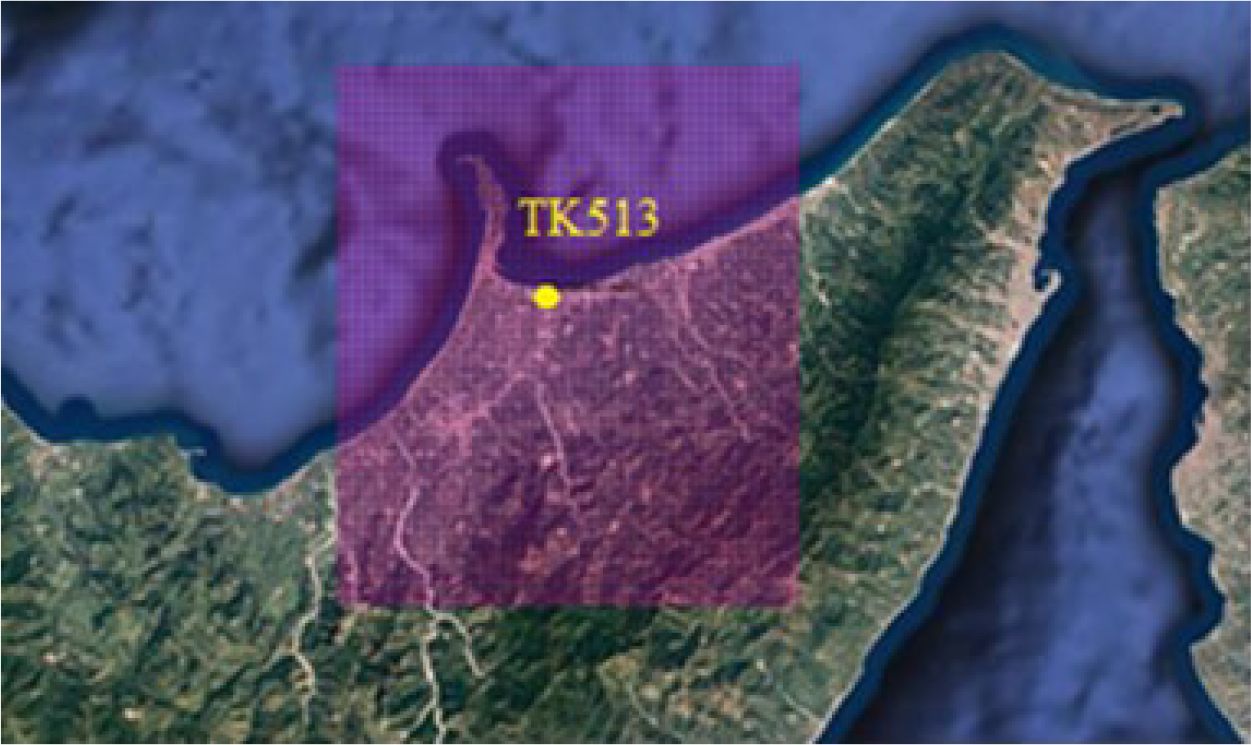
The fire started in one of the storage tanks (TK513 in Figure 2) filled with virgin naphtha, at around midnight. The virgin naphtha burned for approximately 10 hours, releasing pollutants into the atmosphere [25].
Map of the “Mediterranea” refinery.
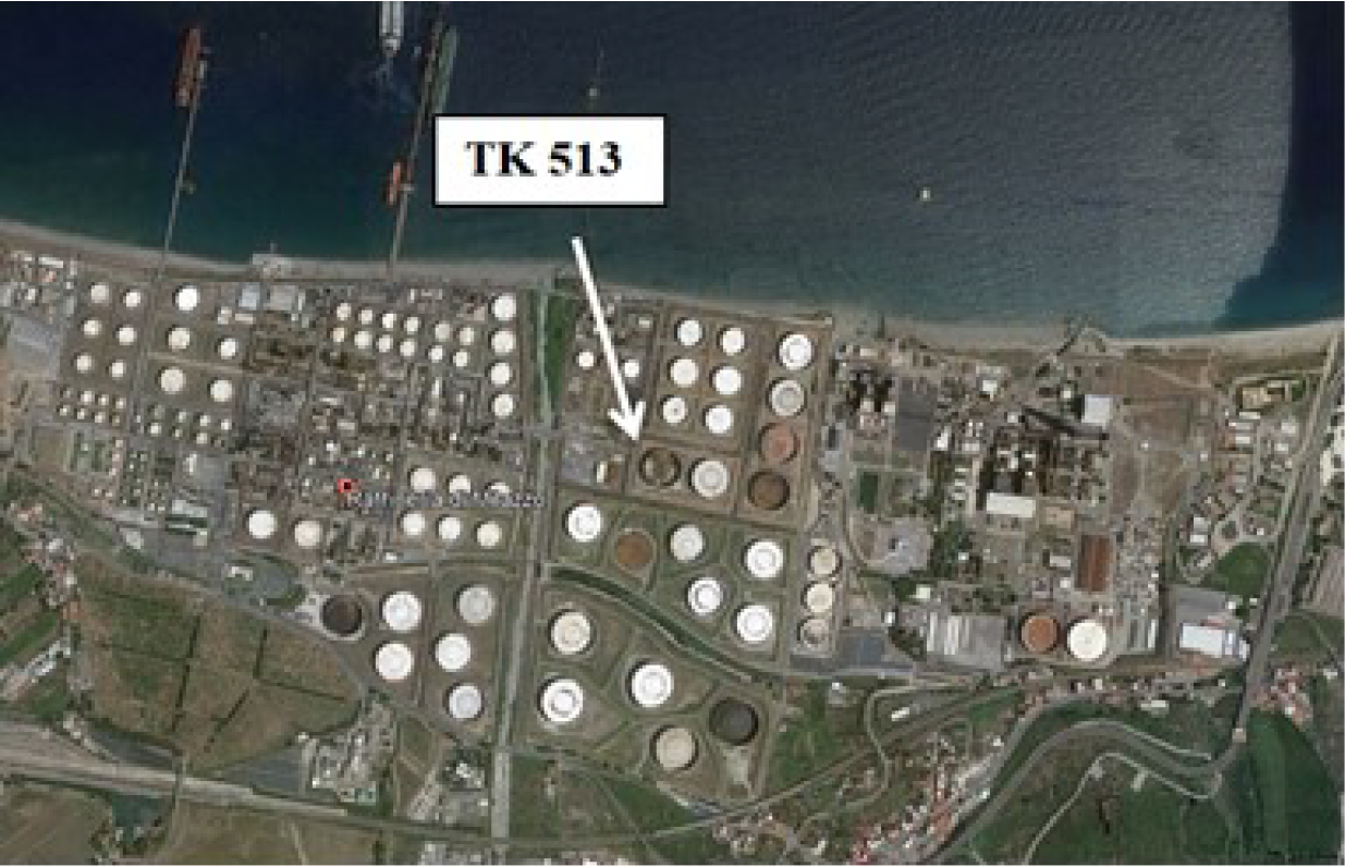
A failure of the floating roof sealing system in the storage tank TK513 caused fuel oil vapour emissions into the atmosphere and conditions favourable to triggering fires. Moreover, the safety device designed to transfer virgin naphtha from storage tank TK513 to other storage systems functioned only partially because some pumps were out of service, probably for maintenance.
The facility operator declared that the storage tank was filled with less than half of its nominal volume (50,000 m3) before the accident [25]. Since the information about the initial and boundary conditions of the incident was not sufficient to provide a thorough description of the chain of events, the analysis was performed as the “worst-case scenario”.
Comparisons between CALMET/CALPUFF simulations based on data elaborated with FORCALM and simulations carried out with observed meteorological data are described in the following section.
The domain used for this study was a grid with an extension of 23 × 27 km, with a cell spacing of 0.5 km, as shown in Figure 1. Optimisation of CALMET input parameters was achieved on the basis of a preliminary analysis of the orographic complexity of the domain under study.
In particular, attention was paid to choose of the parameter called TERRAD, which is specified by the user. TERRAD is related to the highest gridded terrain height within a radius of influence used by the CALMET model to compute the following parameters [16]: kinematic effects of terrain, slope flow effects and blocking effects on the wind field.
Analyses performed using QGIS software about ridge-to-ridge distances across hills of neighbouring cells allowed an evaluation of TERRAD value of 2.5 km.
Moreover, some parameters of the CALMET model were set according to the guidelines included in the U.S. EPA [26], [27]. For simulations based on weather station observations, data were provided by the Servizio Informativo Agrometeorologico Siciliano (SIAS) network consisting of 60 surface stations, with instruments to measure atmospheric conditions at 2 and 10 m; 13 surface stations of World Meteorological Organization (WMO) network; 4 surface stations of Mareografica network; and 1 upper-air station located in Trapani-Birgi airport.
This level of detail allowed improving the quality and accuracy of the simulations and consequently a better comparison with the results obtained using FORCALM. With regard to the definition of parameters used in CALPUFF input, a preliminary study was carried out to model the Milazzo fire as resulting from a large puddle of fuel oil, in uncontrolled conditions [28]. The pollutant mass flow rates used for all simulations are reported in Table 1 as indicated in [29].
Pollutants emitted by the source area, used for CALPUFF simulations
| Pollutant | [kg/s] |
|---|---|
| CO2 | 1184.3 |
| CO | 41.2 |
| NOx | 1.6 |
| VOC (Volatile Organic Compounds) | 2.1 |
| PAH (Polycyclic Aromatic Hydrocarbons) | 59.2 |
| SO2 | 10.0 |
| PM (Particulate Matter) | 59.2 |
Figure 3through Figure 11 report comparisons between CALMET/CALPUFF simulations obtained using FORCALM and results derived by using observed meteorological data, covering a large area of the Sicily region for the period under consideration.
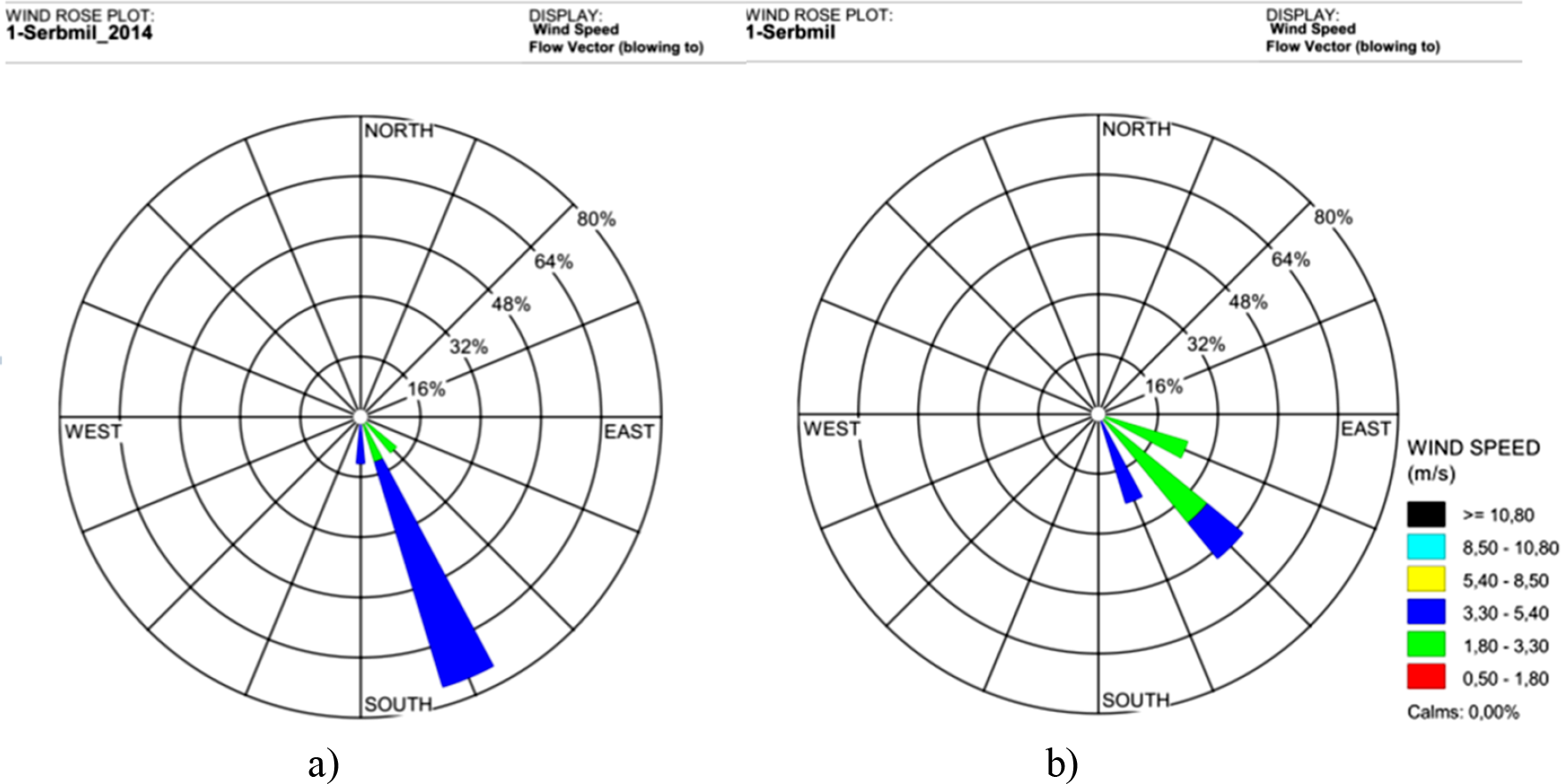
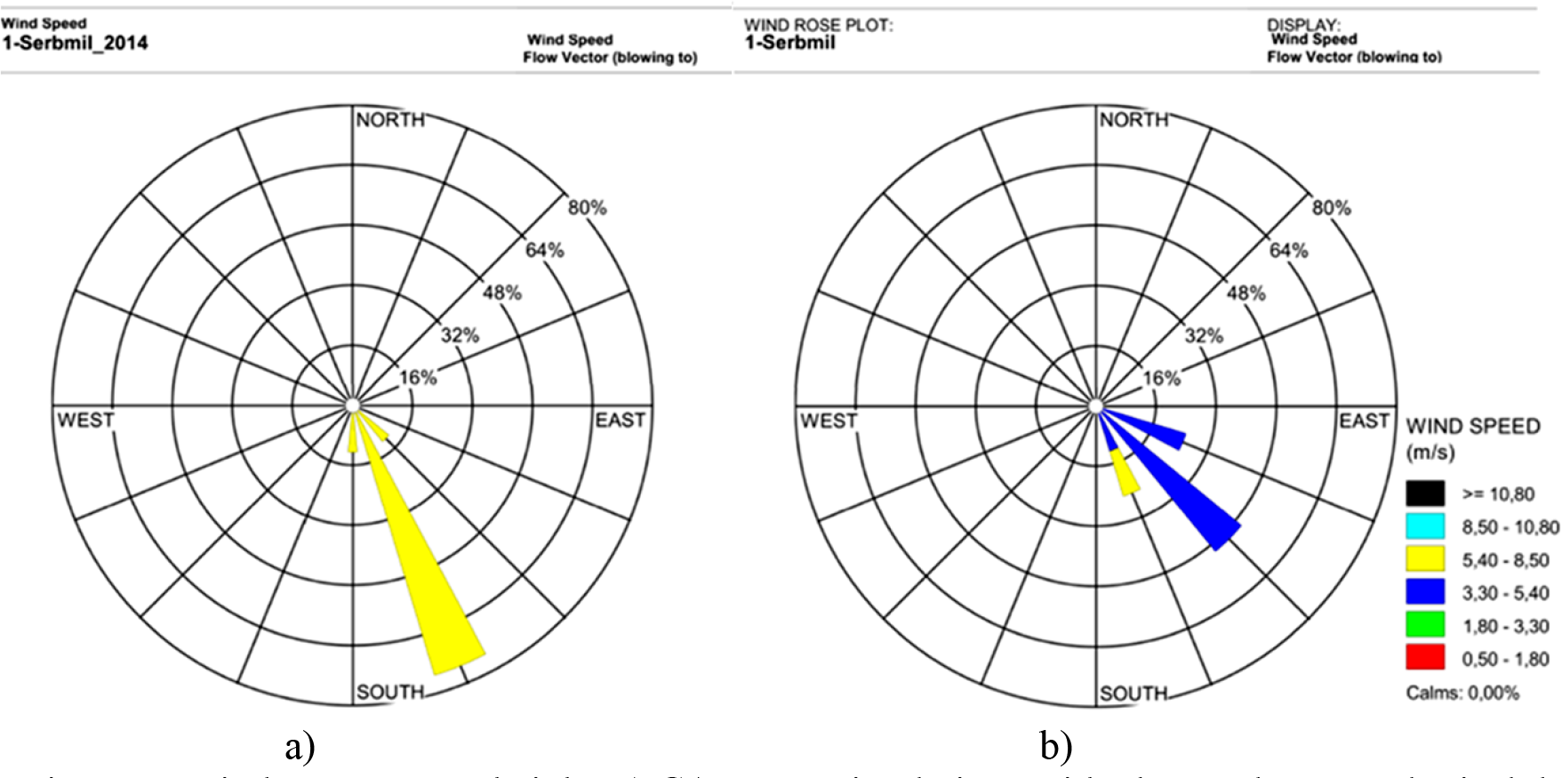
Wind rose at 10 m height: a) CALMET simulations with observed meteorological data; b) CALMET simulations with ECMWF data elaborated with FORCALM tool.
Wind rose at 20 m height: a) CALMET simulations with observed meteorological data; b) CALMET simulations with ECMWF data elaborated with FORCALM tool.
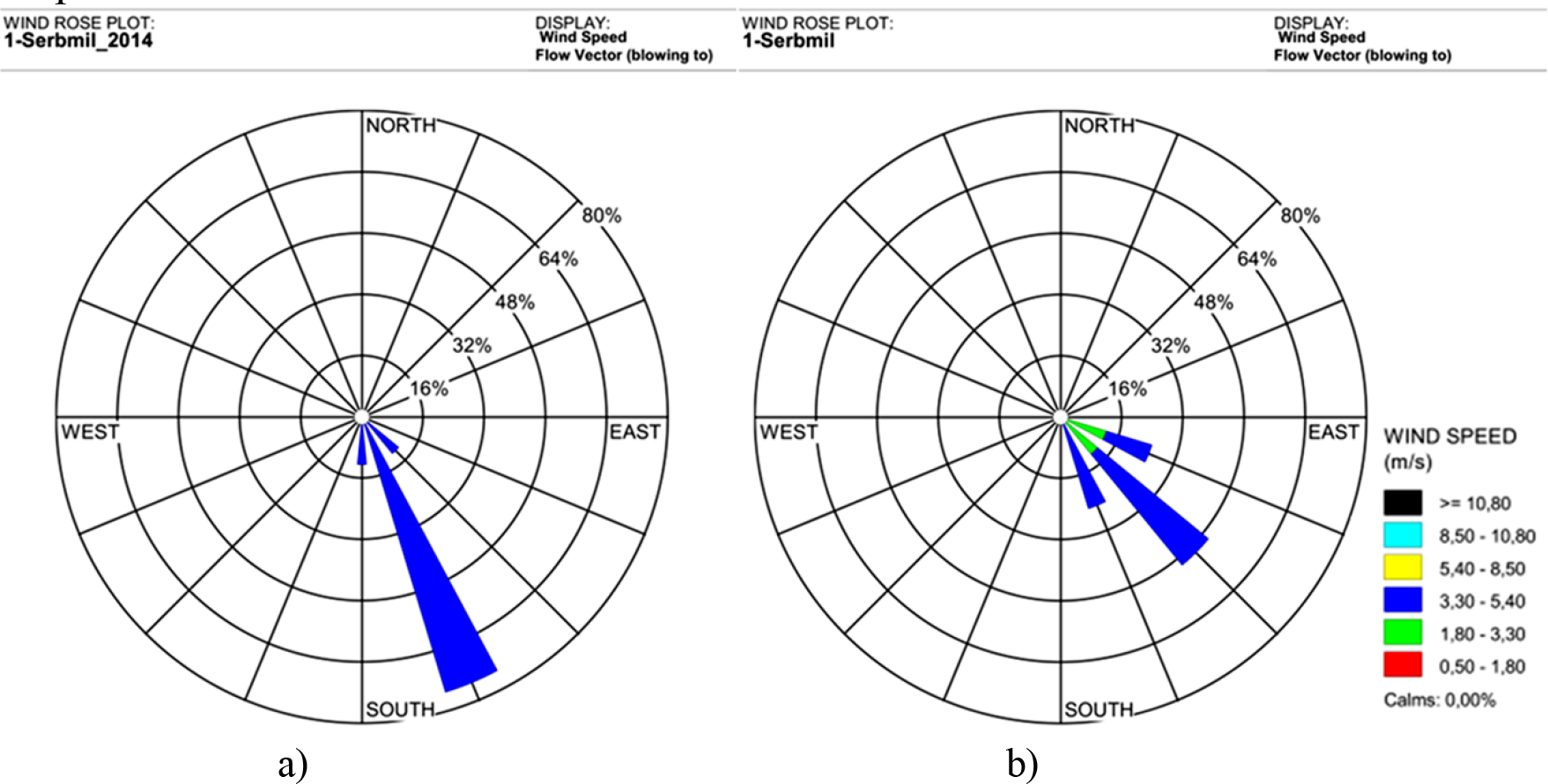
Wind rose at 40 m height: a) CALMET simulations with observed meteorological data; b) CALMET simulations with ECMWF data elaborated with FORCALM tool.
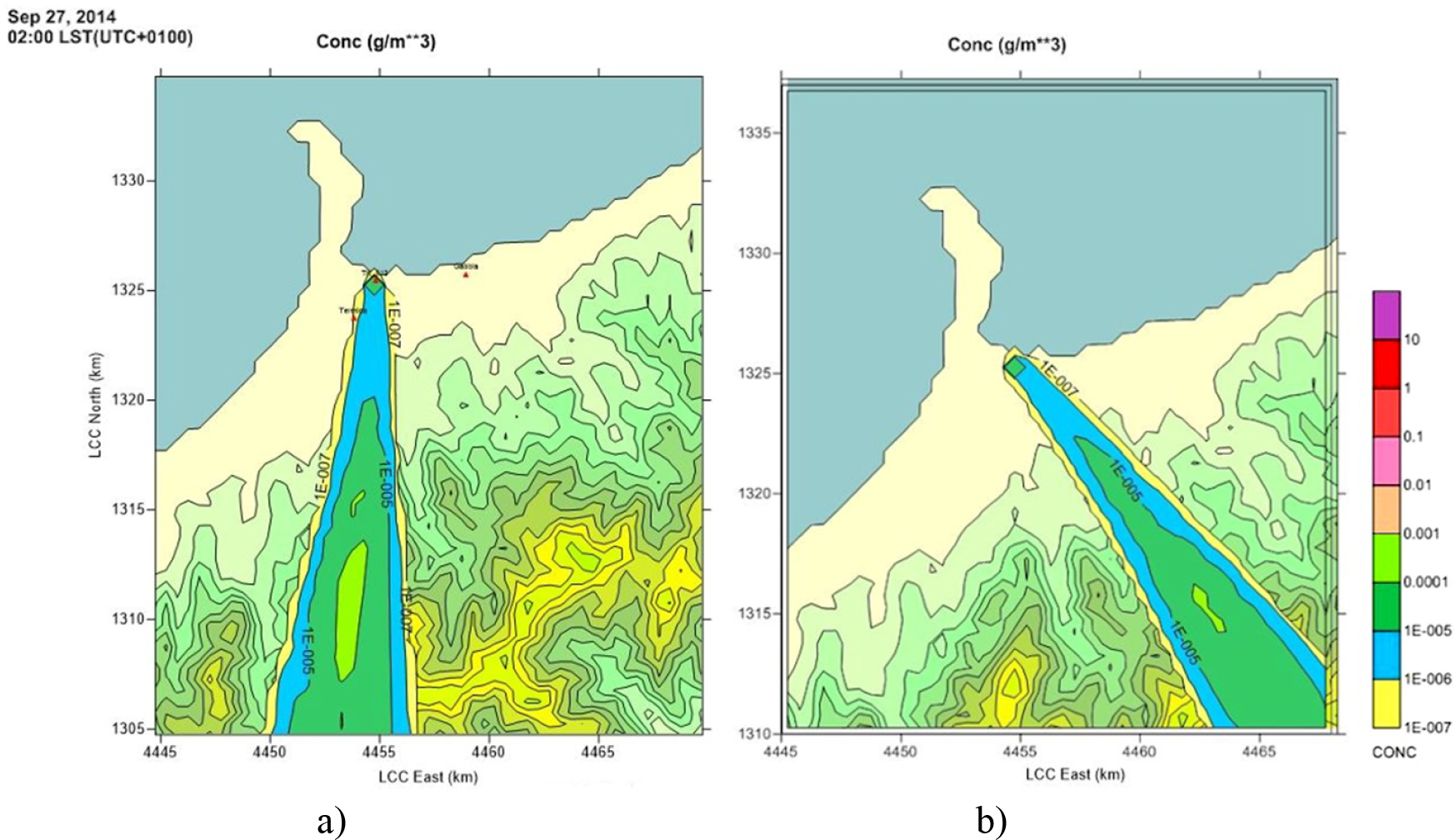
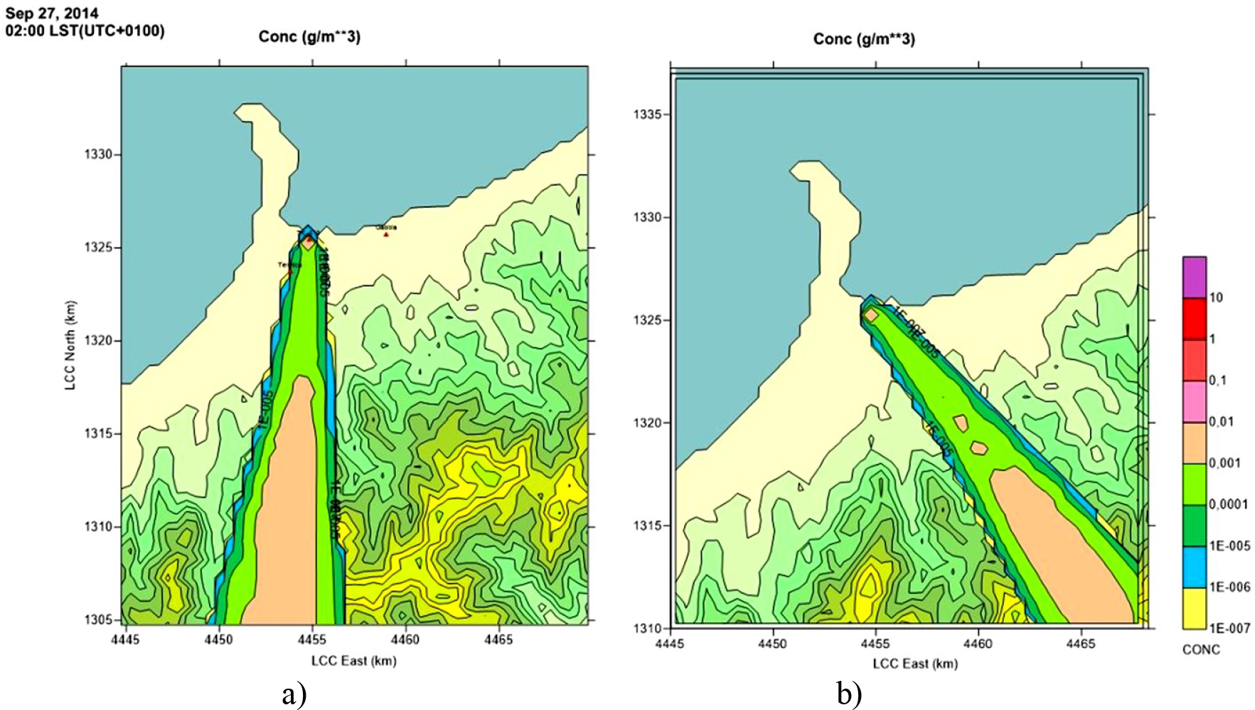
Spatial distribution of NOx at 40 m above ground level, at 2.00 am: a) CALMET/ CALPUFF results by using observed meteorological data; b) FORCALM results.
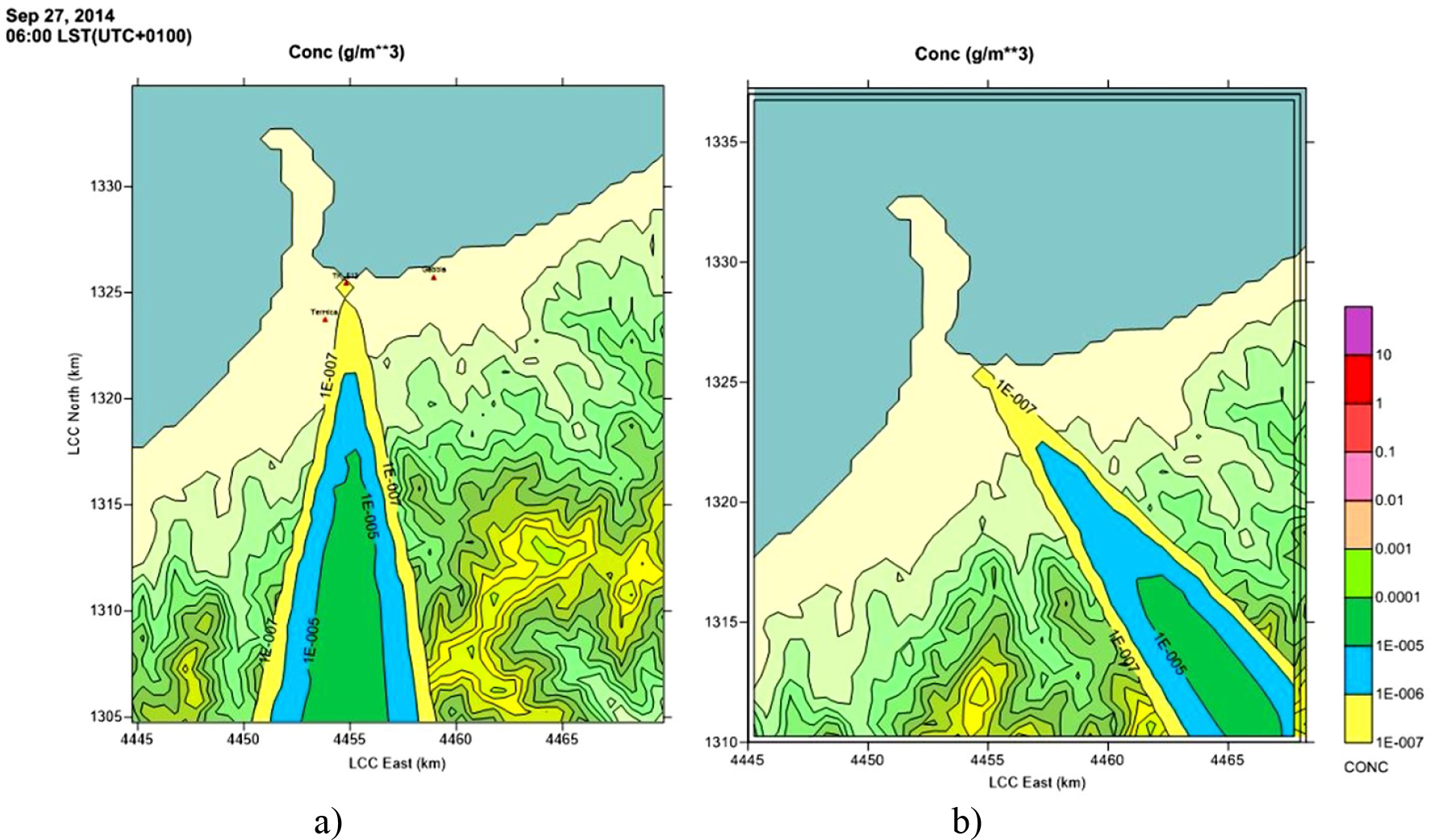
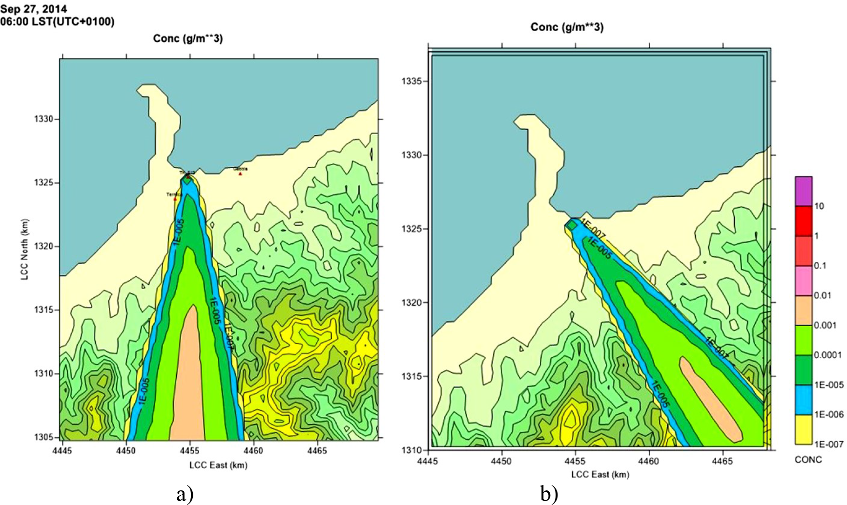
Spatial distribution of NOx at 40 m above ground level, at 6.00 am: a) CALMET/ CALPUFF results by using observed meteorological data; b) FORCALM results.
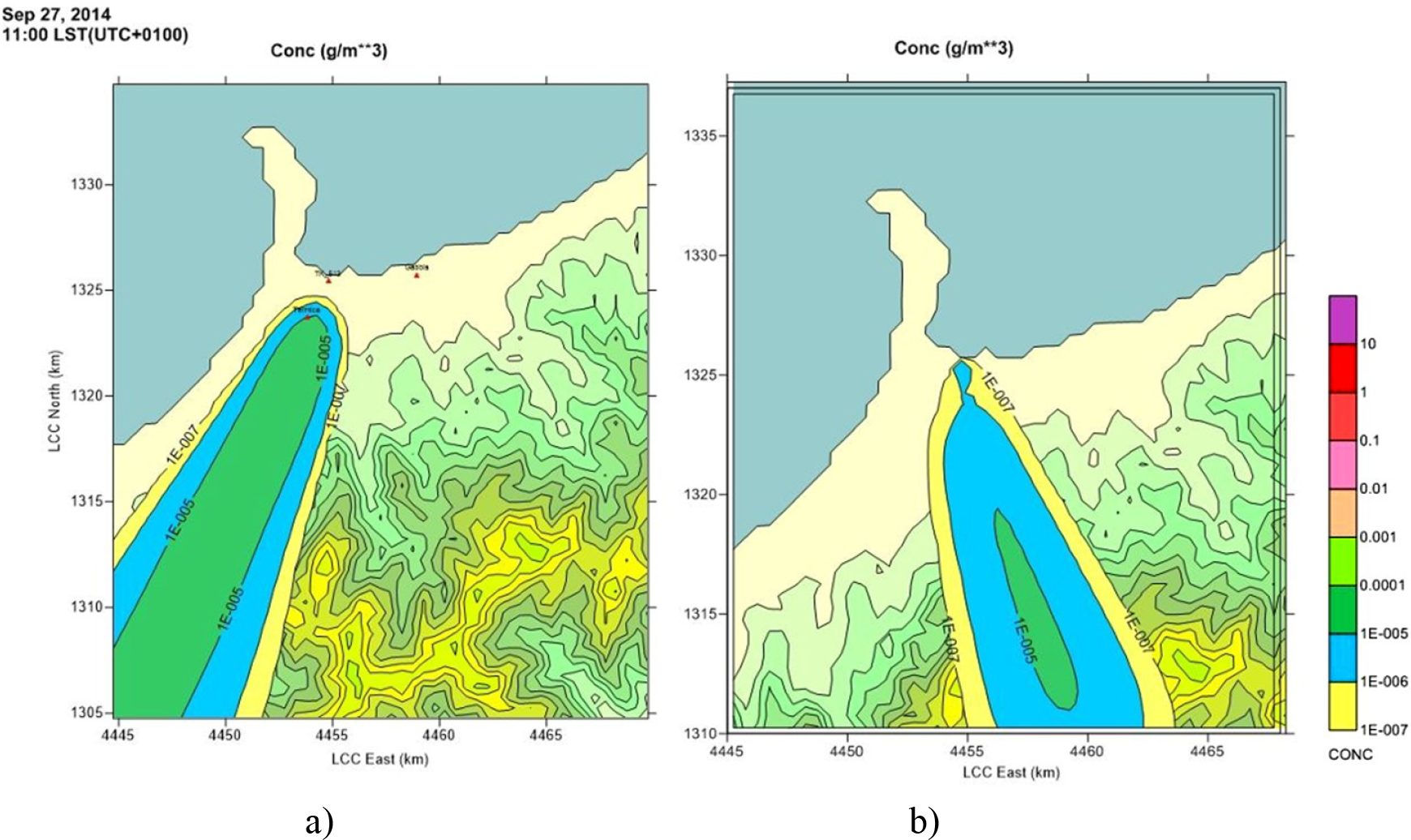
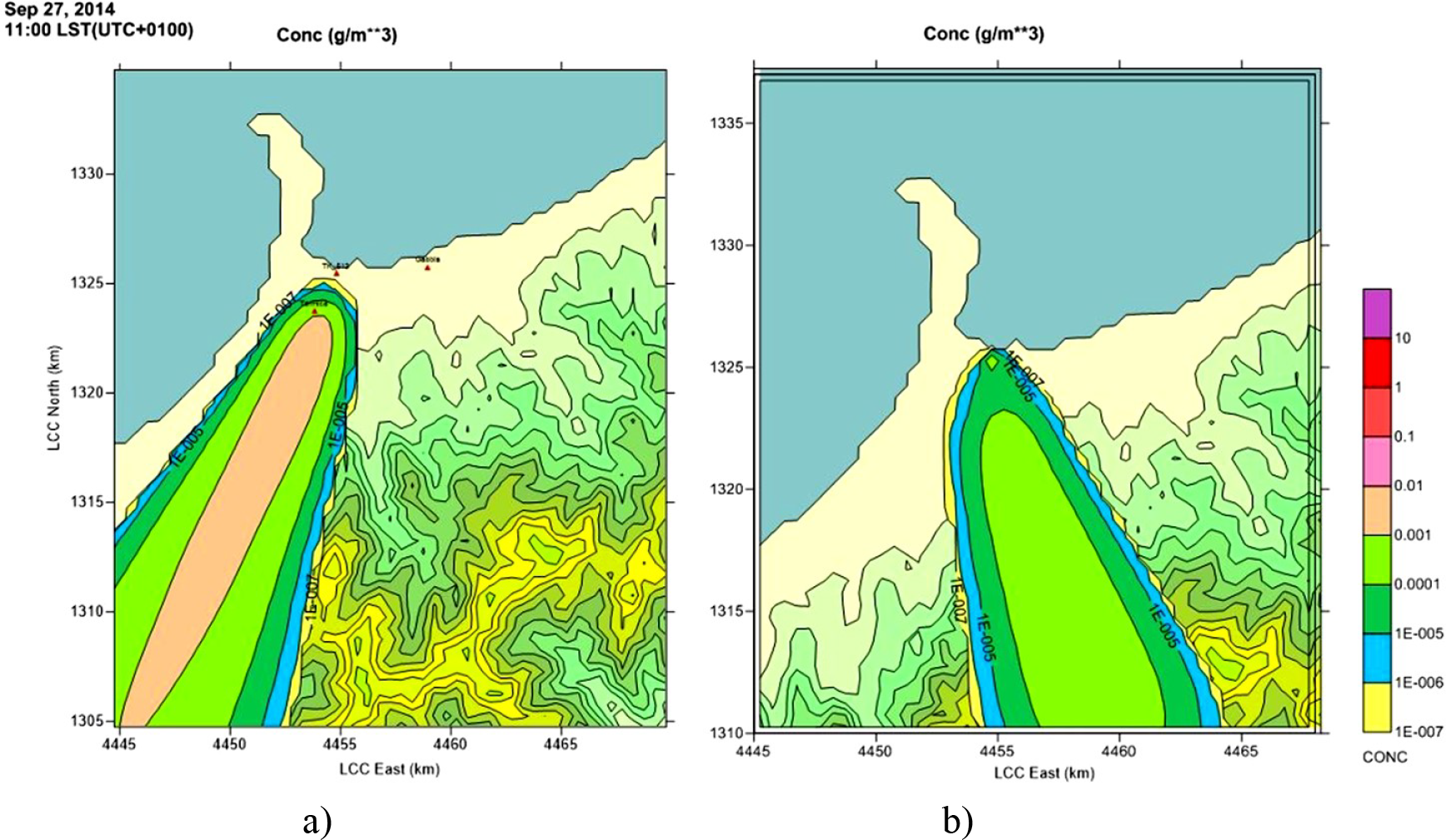
Spatial distribution of NOx at 40 m above ground level, at 11.00 am: a) CALMET/ CALPUFF results by using observed meteorological data; b) FORCALM results.
Spatial distribution of PAH at 40 m above ground level, at 2.00 am: a) CALMET/ CALPUFF results by using observed meteorological data; b) FORCALM results.
Spatial distribution of PAH at 40 m above ground level, at 6.00 am: a) CALMET/ CALPUFF results by using observed meteorological data; b) FORCALM results.
Spatial distribution of PAH at 40 m above ground level, at 11.00 am: a) CALMET/ CALPUFF results by using observed meteorological data; b) FORCALM results.
Results in terms of wind roses, extracted at 10, 20 and 40 m height in the cell where storage tank TK513 is located, are reported in Figure 3 through Figure 5, respectively. Overall, wind rose comparisons highlight the following aspects:
Directional features of the wind fall within the same quadrant (i.e. fourth quadrant, South-East area) with a difference of about 25° at all heights above ground level (Figure 3 through Figure 5).
At heights of 10 and 20 m above ground level, very close wind speed classes are obtained (Figure 3 and Figure 4);
At the height of 40 m above ground level, CALMET predictions with observed meteorological data (Figure 5a) show higher wind speeds than predictions obtained by using FORCALM (Figure 5b), although wind speed classes are close to each other.
In particular, wind roses extracted at 10 and 20 m show close results in terms of wind speed of class of 3.3÷5.4 m/s. Moreover, for this class, it is noticed that a frequency close to 70% for simulation with observed meteorological data (see Figure 3a and Figure 4a) compared to a frequency close to 50% for simulation obtained using FORCALM (see Figure 3b and Figure 4b).
For wind roses extracted at 10 m as in Figure 3, wind speed of class 1.8÷3.3 m/s (low wind speed) is present in both the simulations; however, the result obtained using FORCALM shows the highest frequency.
For wind roses extracted at 20 m as in Figure 4, simulation elaborated with FORCALM (Figure 4b) shows wind intensity of class 1.8÷3.3 m/s with very low frequency (less than 16%), and the two simulations appear to be very close. For wind rose extracted at 40 m as in Figure 5, simulation elaborated with FORCALM (Figure 5b) shows two classes of wind speed (i.e. 3.3÷5.4 and 5.4÷8.5 m/s), whereas simulation with observed meteorological data reports only one class of wind speed, i.e. 5.4÷8.5 m/s (Figure 5a). However, it is worth noting that these wind speed classes are close to each other.
As regards results obtained by using the CALPUFF model, for the sake of brevity, only spatial dispersion data of NOx and PAH at 40 m above ground level are reported at 2:00 am, 6:00 am and 11:00 am on 28th September 2014.
Figure 6through Figure 8 report results for NOx, and Figure 9 through Figure 11 report results for PAH. It can be noted that the plume dispersion for both simulations follows the same direction of rotation, with the passing of the hours.
Moreover, as expected, displacement of about 25° was preserved, coherent with the results in terms of wind roses as described above. This outcome allows the assertion that FORCALM leads to predicting the wind’s dynamic aspects and producing a real-time plume with considerable accuracy. Distribution values of NOx, as reported in Figure 6 and Figure 7 at 2:00 am and 6:00 am in the simulation, show that the concentrations are very close to each other, especially for the highest concentration ranks (i.e. 0.001÷0.0001 g/m3 and 0.0001÷0.00001 g/m3).
With regard to the results relevant to the distribution of PAH, comparisons are very close for all the considered simulation times (Figure 9 ÷ Figure 11).
Further, it is interesting to note that plume transport and its spread as a function of time, obtained by the simulation elaborated with FORCALM, agree with the results obtained using observed data.
During the 10 hours of the accident, several videos were captured of the fire as seen from the sea area – near the Palermo-Messina motorway and Milazzo town. On the basis of these images, it was possible to reconstruct and examine the time- and direction-based development of the plume.
The observation verified the formation of a black smoke plume with an altitude of about 1500 m. Due to its high buoyancy, the plume rose vertically upwards and transported most of the plume material clear of the boundary layer. The results of both simulations reflect what was recorded.
The FORCALM tool was developed at the Engineering Department, University of Palermo (Italy), to elaborate the European Centre of Medium-Range Weather Forecasts data on a 3D grid with high resolution and to be used for specialised atmospheric dispersion-modelling techniques. The aim was to identify risk levels in case of severe accidents and support the strategic tools of emergency response plans and forecast-based actions to select appropriate response options.
It is worth noting that most of the studies carried out so far have been based on the assumption that learning from past events is the suitable way to learn to handle an emergency. However, this approach may be less effective if the chain of events manifests itself in ways different from past events.
In this context, FORCALM can handle forecast meteorological data to be used in transport, dispersion, and deposition analyses of airborne pollutants to enable advance responses to emergency situations over short or long periods of time.
The validation activity concerns a case study related to the accident that occurred at the “Mediterranea” refinery in Milazzo (Sicily, Italy) on 28 September 2014. The area bordering the refinery is characterised by a particularly complex orography, with the sea to the north of Milazzo and the Peloritani Mountains located to the south. The fire started at around midnight in one of the storage tanks filled with virgin naphtha, burning for approximately 10 hours and causing the release of pollutants into the atmosphere. Comparisons were performed between CALMET/CALPUFF simulations obtained using data of the ECMWF elaborated by FORCALM and analyses carried out with observed meteorological data covering the Sicily region. The results in terms of wind roses and plume dispersions of NOx and PAH, as reported in this paper, reveal that assessments carried out by using FORCALM provide information about the potential impacts with a considerable degree of accuracy.
In particular, it can be noted that the plume dispersion follows the same direction of rotation with time for both simulations. Moreover, a displacement of about 25° is preserved, coherent with the results related to wind roses. It is interesting to note that plume transport and its spread as a function of time, obtained by using forecast meteorological models of FORCALM, agree with the results obtained using observed meteorological data. The results of this study suggest that the use of FORCALM is promising for the formulation of emergency response plans and forecast-based actions.
The authors would like to acknowledge the use of ECMWF weather data for the simulations performed.
- ,
Safety study of an LNG regasification plant using an FMECA and HAZOP integrated methodology ,J. Loss Prev. Process Ind. , Vol. 35 ,pp 35–45 , 2015, https://doi.org/10.1016/j.jlp.2015.03.013 - , Measuring Territorial Vulnerability? An Attempt of Qualification and Quantification, Lect. Notes Comput. Sci. (including Subser. Lect. Notes Artif. Intell. Lect. Notes Bioinformatics), 2014
- ,
Fuzzy environmental analogy index to develop environmental similarity maps for designing air quality monitoring networks on a large-scale ,Stoch. Environ. Res. Risk Assess. , Vol. 33 (10),pp 1793–1813 , 2019, https://doi.org/10.1007/s00477-019-01723-w - ,
Risk and resilience: strategies for security ,Civ. Eng. Environ. Syst. , Vol. 32 (June),pp 100–118 , 2015, https://doi.org/10.1080/10286608.2015.1023793 - ,
Development of a decision support system for assessing the supply chain risk mitigation strategies: an application in Indian petroleum supply chain ,J. Manuf. Technol. Manag. , Vol. 32 (2),pp 506–535 , 2020, https://doi.org/10.1108/JMTM-02-2020-0035 - ,
Contingency Planning Emergency Response and Safety ,Introduction to Security , Vol. 2507 (February),pp 1–9 , 2019 - ,
A resilience engineering approach for sustainable safety in green construction ,J. Sustain. Dev. Energy, Water Environ. Syst. , Vol. 5 (4),pp 480–495 , 2017, https://doi.org/10.13044/j.sdewes.d5.0174 - ,
Analysis of accidents in biogas production and upgrading ,Renew. Energy , Vol. 96 ,pp 1127–1134 , 2016, https://doi.org/10.1016/j.renene.2015.10.017 - ,
A new approach for modeling dry deposition velocity of particles ,Atmos. Environ. , Vol. 180 (February),pp 11–22 , 2018, https://doi.org/10.1016/j.atmosenv.2018.02.038 - ,
Dry deposition models for radionuclides dispersed in air: A new approach for deposition velocity evaluation schema ,J. Phys. Conf. Ser. , Vol. 923 (1),pp 0–11 , 2017, https://doi.org/10.1088/1742-6596/923/1/012057 - ,
Atmospheric dry deposition processes of particles on urban and suburban surfaces: Modelling and validation works ,Atmos. Environ. , Vol. 214 (July), 2019, https://doi.org/10.1016/j.atmosenv.2019.116857 - ,
Validation of numerically forecast vertical temperature profile with measurements for dispersion modelling ,Int. J. Environ. Pollut. , Vol. 64 (1/2/3),pp 22 , 2018, https://doi.org/10.1504/ijep.2018.10020560 - ,
Forecasting lightning around the Korean Peninsula by postprocessing ECMWF data using SVMs and undersampling ,Atmos. Res. , Vol. 243 (May),pp 105026 , 2020, https://doi.org/10.1016/j.atmosres.2020.105026 - ,
A refined regional model for estimating pressure, temperature, and water vapor pressure for geodetic applications in China ,Remote Sens. , Vol. 12 (11),pp 1–20 , 2020, https://doi.org/10.3390/rs12111713 - ,
An LSTM-based aggregated model for air pollution forecasting ,Atmos. Pollut. Res. , Vol. 11 (8),pp 1451–1463 , 2020, https://doi.org/10.1016/j.apr.2020.05.015 - ,
Uncertainties in atmospheric dispersion modelling during nuclear accidents ,J. Environ. Radioact. , Vol. 222 (March), 2020, https://doi.org/10.1016/j.jenvrad.2020.106356 - ,
A modeling study of PM2.5 transboundary transport during a winter severe haze episode in southern Yangtze River Delta, China ,Atmos. Res. , Vol. 248 (February 2020), :1051592021, https://doi.org/10.1016/j.atmosres.2020.105159 - ,
A user’s guide for the CALMET meteorological model ,Renew. Sustain. Energy Rev. , (January),pp 1–332 , 2000 - ,
A User’s Guide for the CALPUFF Dispersion Model ,Lem.Org.Cn , (January), 2000 - , , FUNDAMENTALS OF ATMOSPHERIC MODELING, 2005
- ,
A COORDINATE SYSTEM HAVING SOME SPECIAL ADVANTAGES FOR NUMERICAL FORECASTING ,J. Atmos. Sci. , Vol. 14 (2),pp 184–185 , 1957, https://doi.org/10.1175/1520-0469(1957)014%3C0184:ACSHSS%3E2.0.CO;2 - ,
, U.S Standard Atmospher , 1976 - ,
, Hydrology for Engineers , 1982, Subsequent - ,
, Atmospheric Thermodynamics , 2012 - ,
, Virgin Nafta fire in TK513 storage tank od Milazzo’s refinery - model analysis foe the assessment of combustion fumes dispersion , 2015 - , , Interagency workgroup on air quality modeling (IWAQM) phase 2 summary report and recommendations for modeling longrange transport impacts, 1998
- , , Reassessment of the Interagency Workgroup on Air Quality Modeling (IWAQM) Phase 2 Summary Report: Revisions to Phase 2 Recommendations, 2016
- ,
Observations of the plume generated by the December 2005 oil depot explosions and prolonged fire at Buncefield (Hertfordshire, UK) and associated atmospheric changes ,Proc. R. Soc. A Math. Phys. Eng. Sci. , Vol. 463 (2081),pp 1153–1177 , 2007, https://doi.org/10.1098/rspa.2006.1810 - ,
Modelling pollutants dispersion and plume rise from large hydrocarbon tank fires in neutrally stratified atmosphere ,Atmos. Environ. , Vol. 44 (6),pp 803–813 , 2010, https://doi.org/10.1016/j.atmosenv.2009.11.034