


In the last few years, the European Commission has set various ambitious targets in order to reduce CO2 emissions. As a result of this, the Dutch government has been regulating the energy sector to move towards the use of green energy in order to avoid the use of natural gasses completely by the end of 2050 [1]. Moreover, in The Netherlands, there has been a growing concern with the use of natural gas, because of the exponential growth of earthquakes caused by the extraction of gas from the Groningen gas field. Accordingly, the urgency of reducing the use of natural gasses in dwellings is growing strongly. Although most energy in The Netherlands is used by industry, the build environment is responsible for 28% of the energy use of which 71% is for heating purposes. Currently, 87% of the buildings heating energy needs are covered with the use of natural gas [2]. Technologies that currently exist which could help to reduce the use of natural gasses, are easier to implement in the build environment rather than the industry, since the industry often has higher temperature needs than the build environment [3] [4].
To reduce the use of gas in the built environment, several new and renovated dwellings have already been constructed to Net-Zero Energy Building (NZEB) standard [5] [6]. This means that for these dwellings the total amount of energy used on an annual basis is equal to the amount of renewable energy created on site. The type of energy produced and used by these types of dwellings in The Netherlands is only electrical [7]. The electricity energy use and production patterns of NZEB dwellings differs a great deal from the average dwelling, because of the variety of heating and energy producing systems used [8].
Since these dwellings have such different energy patterns, new approaches are needed to be able to take technical/political decisions on what type of technologies to promote. Government-organisations are in need of this information when creating/improving (existing) policies concerning the NZEB standard. To establish these policies, new innovation is needed to collect data about dwelling energy usage and delivery, which can be collected from the dwellings itself. A good technique for collecting this information is through smart meters.
By 2020, 80% of the households in The Netherlands will have a smart meter. A smart meter measures the amount of energy taken from and sent to the net [9] [10]. This data, in combination with publicly available data, could allow determining dwelling characteristics and the energy use behaviour of its residents. This information could be used to optimize the current dwellings energy systems, gain more knowledge about energy use patterns and propose possible improvements with the goal to reduce CO2 emissions related to energy use [11].
Previous research shows insights about household electricity consumption and CO2 emissions on dwellings in The Netherlands. It explores the effect of smart meter, appliance efficiency, and consumer behaviour on reducing electricity consumption in The Netherlands. The results show their effect on electricity consumption and suggest that further effort is required to control and reduce it. Insights from the paper suggest that future studies should disaggregate with respect to several factors in electricity consumption, as George Papachristos has stated in his paper [12].
Based on the research of Papachristos, behavioural patterns have been formed based on the characteristics of dwellings and electricity consumption. It analyses the appliance uses in the Dutch housing stock and define behavioural patterns and profiles of electricity consumption in detail. This has been done with survey data which were collected from 323 dwellings in The Netherlands on appliance ownership and use of electricity [13].
Currently, smart meters are being installed in most of the Dutch dwellings. Data from the smart meters contains important information about the minimum and maximum amount of energy circling back and forward in the net. This is needed to change the current net infrastructure because the current infrastructure is not built for receiving as much energy from dwellings. Energy produced at dwellings should be able to be sent back to the net without little to no energy loss. This energy can then be used at moments without sun and/or wind [14].
Thorough analysis of 15-minute residential smart meter datasets, it is possible to identify possible value propositions of smart meter measurements. The results showed that for different applications, the communication needs from meters to control-centers, data storage capabilities, and the complexity of data processing intelligence varies significantly [15].
When introducing the people in the dwelling with their consumer behaviour, this can be used to change their behaviour and therefore reduce the yearly energy cost. The consumption behaviour is based on the amount of energy every device in the dwelling is using, visualized by logistic regression machine learning [16]. Another research proves that the use of machine learning algorithms can be used to forecast residential gas consumption based on energy consumption data and weather data. Gaining insight into the energy consumption with machine learning algorithms can be helpful in balancing the grid and insights in how to reduce the energy consumption can be received [17] [18]. Furthermore, machine learning algorithms can also predict energy demand on specific time-period [19].
This research focuses on gaining insights on the dwelling characteristics by using machine learning algorithms on smart meter data in combination with weather data. Specifically, the paper compares the accuracy of the models.
In the following chapters, a comprehensive analysis and pre-processing of the provided smart meter data are covered, including the implementation of different machine learning algorithms. The generated models were then validated and evaluated using evaluation metrices, which are compared in the results.
Supervised machine learning and neural network methods have been used in this research. Machine learning has proven to be a solution to different problems, including when it comes to analysing smart meter data [17] [20]. Logistic Regression, Support Vector Machine, and K-Nearest Neighbors are some one of the most used machine learning algorithms today. These algorithms are hardly been used to classify smart meter data; however, they are commonly used to work efficient with the classification of sequential data [21]. In addition to supervised machine learning, neural networks show vastly promising results when predicting/classifying data with regards to the process of producing and consuming energy [22]. Recurrent Neural Network is a type of neural networks, which are designed to detect and recognize patterns in sequences of data. All these algorithms are described in their respective subsections.
Furthermore, the data collecting and pre-processing methods used are described as well as the classification metrics to evaluate the effectiveness and performance of the different machine learning models. This section also specifies the used environmental settings for all the models. All the analysis and modelling were done in Python.
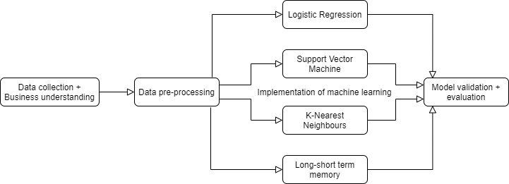
Figure 1 shows a flowchart with the different methods performed during this research.
Flowchart with the performed methods within this research
The original dataset that was used during this research consists of an Excel-file with two sheets. This file contains records in the form of time series of energy delivery and consumption data from 33 dwellings of a neighbourhood called Groene Mient in The Netherlands. The data was extracted from the smart meters installed in these dwellings. The smart meters collected energy delivery and consumption records from 11-07-2017 till 31-05-2019. The data exists of the amount of kWh (kilowatt-hour) taken from the net, and the amount of kWh going back to the net minus the consumption of the residents. This is measured and stored every 15 minutes. The smart meter measures the use of energy in kWh. The dwelling characteristics are manually added to the dataset by their rightful owners. These characteristics divide into three parts. The first one is the type of heating system installed in the dwelling. This can either be represented as ‘E’ (net energy), ‘WP’ (heating pump) and ‘Zon’ (thermal solar panel). The second one is the number of solar panels. These can vary between 8 and 17. The third one is the number of inhabitants. This can vary between 1 and 4. Dwelling characteristics come in many varieties, however due to constrains in the data availability and confidentiality reasons, only the three characteristics mentioned above were made available by the Groene Mient and used during this research. Furthermore, it is good to address that the only energy source for producing the renewable energy comes for the solar panels installed on each dwelling. Additional needed energy is collected from the Dutch energy supplier.
In the data cleaning phase, the Python-scripts pre-processed the rows containing missing records and accumulated consumption data so that correct learning models could be created in the next phase. The dataset consists of different data depending on each dwelling because the smart meters were installed at different times. Therefore, the dataset was reduced for the dwellings which had fewer data compared to the other dwellings. This process cleaned out five dwellings from the dataset, which means that every machine learning model was built based on the 28 dwellings that were left in the dataset.
Apart from the smart meters data, weather data has been gathered from the Koninklijk Nederlands Meteorologisch Instituut (KNMI) [18]. This dataset helps us to build the models providing more data about the environment which influence directly to the energy delivery and consumption. The data consists of the temperature, duration of sunshine, global radiation and cloud cover indexes. Moreover, dummy variables, variables that are created from values within the dataset, have been created based on the timestamps, including are the following: hour of the day, day of the week, day of the month, week of the month, month and season.
In order to let the algorithms find the underlying patterns to correctly predict the targets, it is necessary to perform a transformation of the original dataset by grouping the energy delivery and consumption into series of daily and weekly data. Depending on which aggregated data an algorithm is trained with, it always predicted better with aggregated data instead of data per 15 minutes. For the weather data, the mean has been computed of every variable during the week, and for the dummy variables, the mode has been calculated. In the case of the Recurrent Neural Network, this grouping was not necessary to do.
Machine learning is an evolving branch of computational algorithms that are designed to emulate human intelligence by learning from the surrounding environment. They are considered the working horse in the new era of the so-called big data. Machine learning can be divided according to the nature of the data labelling into supervised, unsupervised, and semi-supervised. Supervised learning is applicable for estimating an unknown (input, output) mapping from known (input, output) samples, where the output is labelled (e.g. classification and regression). While in unsupervised learning, only input samples are given to the learning system (e.g. clustering and estimation of probability density function) [23].
The focus was on supervised learning because it allows to classify different targets, including which type of heating system, number of solar panels and number of inhabitants is the most suitable for a certain dwelling by using the available datasets. This is done by using classification algorithms, which classify data into two or more classes.
The following machine learning algorithms have been used in order to classify based on the data:
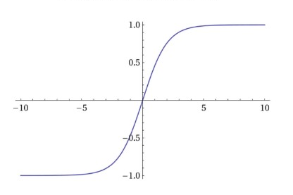
Logistic Regression. Logistic Regression is a supervised machine learning algorithm which can be used to solve classifications problems. Logistic Regression uses a linear equation to calculate a value. The computed value can be anywhere between negative infinity and positive infinity. The output needs to be between 0 and 1 to make the classification. To scale the output to a value between 0 and 1, the sigmoid function is used where ‘z’ is the output value [24]:
When using Logistic Regression, a threshold is specified that indicates at which value the output will be put into one class versus the other class. A threshold with the value 0.5 means that a class with a 50% (or greater) probability will be classified as class2 and a class with a probability less than 50% as class1. Logistic Regression can be divided into binary (where the model classifies the data in two classes) and multi-class classification (where the model classifies the data in two or more classes). Depending on the data, multi-class classification was used since the prediction for each label could be divided in two or more classes.
The model is fed with 9744 rows of aggregated data per day which contains delivery, consumption and KNMI data. Logistic Regression was used to classify what kind of heating system is used, how many solar panels are installed and how many inhabitants are in this dwelling. For every prediction, a different model is used. To improve the accuracy of the model, the hyperparameter ‘C’ can be changed. For small values of C, the regularization strength is increased which will creates simple models that underfit the data. For large values of C vice versa.
K-Nearest Neighbors. K-Nearest Neighbors (KNN) can be used for both classification and regression predictive problems and is a supervised machine learning algorithm. The goal of the algorithm is to learn a function so that given an unseen observation x, h(x) can confidently predict the corresponding output y.
In the classification setting, KNN essentially boils down to forming a majority vote between the K most similar instances to a given “unseen” observation. The similarity is defined according to a distance metric between two data points. The KNN classifier is commonly based on the Euclidean distance between a test sample and the specified training samples. Let xi be an input sample with p features (xi1, xi2, ..., xip), n be the total number of input samples (i=1, 2, ..., n). The Euclidean distance between sample xi and xj is defined as:
The model is fed with 2912 rows of aggregated data per week which contains delivery, consumption and KNMI data. KNN was used to classify what kind of heating system is used, how many solar panels are installed and how many inhabitants are in this dwelling. For every prediction, a different model is used. To improve the accuracy of the model, the hyperparameter ‘n_neighbors’, which determines how many neighbours have to be checked to set the class for the new sample; and ‘p’, which represents the power parameter for the Minkowski metric can be changed [25].
Recurrent Neural Network. Recurrent Neural Network (RNN) is one type of neural networks which are designed to detect and recognize patterns in sequences of data. The dataset from Groene Mient is suitable for RNN, because it contains time and sequential data. That means that the dataset contains temporal dimensions, which is useful for RNN’s. Furthermore, the dataset contains different sizes of sequences with intervals of 15 minutes. The powerful tool of RNN is that they have a certain type of memory, and that is also part of the human brain condition. As they have feedforward connections, they can use the outputs as part of the next input moment after moment [26].
Long short-term memory. Long Short-Term Memory (LSTM) is a recurrent neural network (RNN) architecture that has shown to outperform traditional RNNs on numerous temporal processing task [26].
LSTM is a variant of the RNN maintaining the error more constantly; therefore, they are used to long time series data memorization in order to continue learning over many more time steps than the traditional RNN. One relevant point of the LSTM is that they have a forget gate; using this feature, the network can forget some low-quality patterns and start over others. Basically, LSTM performs better than other recurrent neural networks when the goal is to learn from very long-term data sequences. The ability to forget, remember and update the information make better adjustments one step ahead of RNNs. The input data shape of the LSTM must be three dimensional. The first dimension measures the batch size, the second one measure the time-steps, and the last one dimension measures the number of units in one input sequence [27].
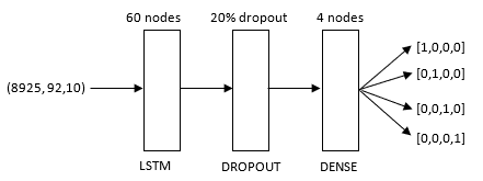
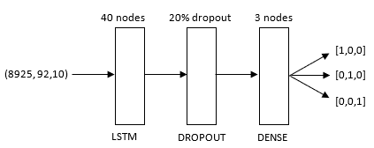
The network is fed with 8925 samples with 92 data records (96 should be the optimum, because there are 92 data records per day, but the entire dataset has no possibility to divide it by 96, so the closest number is 92) and ten units (each data record has ten features to train delivery, consumption, KNMI data and dummy variables).
The architecture of the models in Figure 3 and Figure 4 are composed of three layers. The model in Figure 2 contains an additional dense layer, to intermediately calculate outputs that can be dropped by the dropout layer.
LSTM architecture for classifying the heating system
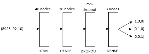
The initial layer consists of a LSTM layer, containing recurrently connected blocks that connect the inputs with multiplicative units. Following is the dropout layer that attempts to remove noise from the data, with the goal to prevent the model from overfitting by forcing the model to learn the pattern in different ways.
This means that their contribution to the activation of downstream neurons is temporally removed on the forward pass and any weight updates are not applied to the neuron on the backward pass) [28]. Finally, the output is another Dense layer using a “softmax” activation function composed of 3 nodes (depends on the number of classes to predict). The outputs of the models are described based on the One-Hot-Encoding (binary encoding). The heating system outputs are encoded as following: [1,0,0] = ”E”, [0,1,0] = “WP”, [0,0,1] = “Zon”. The outputs of the number of inhabitants are encoded as following: [1,0,0,0] = 1 inhabitant, [0,1,0,0] = 2 inhabitants, [0,0,1,0] = 3 inhabitants, [0,0,0,1] = 4 inhabitants. The outputs of the number of solar panels was encoded as following: [1,0,0] = 8-10 solar panels, [0,1,0] = 11-13 solar panels, [0,0,1] = 14-17.
The rectified linear activation function (RELU) is a piecewise linear function that will output the input directly if it is positive. Otherwise, it will output zero defined as following [24]:
By assigning a “softmax” activation function (Figure 5), a generalization of the logistic function, on the output layer of the neural network (or a “softmax” component in a component-based network) for categorical target variables, the outputs can be interpreted as posterior probabilities. This is useful in classification as it gives a certainty measure on classifications.
The "softmax" activation function used in the output "Dense" layer
All the created models using the machine learning algorithms were validated by using Cross Validation. By using Cross Validation, it provides a possibility to assess how the results of a statistical analysis model will generalize to an independent dataset. This is done by splitting up the dataset in a training- and test set with an 80/20 ratio. This is a common approach within machine learning for splitting up data in different sets and is also described as a high-performance measure [29].
The algorithms were trained by the training data. After the training process, the algorithms were validated using the remaining (validation) data. This way, the models are validated on data that it has never seen before. The validation set contains monthly data for the years 2017, 2018 and 2019, where the data is aggregated by a whole day. By extracting the whole day and applying it to the predicted model, the model can give an output of the predicted target. Knowing what the targets are from each dwelling in the validation set, it is possible to validate the predictions with the true targets.
In order to evaluate the models, evaluation metrics were used to produce classification reports that indicates which of the models work the best for this specific problem. The confusion matrix (Figure 6) contains information about actual and predicted classifications done by the classification models. Performance of these models is commonly evaluated using the test data.
The confusion matrix used to determine the performance of the algorithms
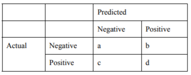
The outputs in the confusion matrix have the following meaning:
The following metrics can be calculated with the outputs of the confusion matrix:
-
Logistic Regression;
-
Support Vector Machine;
-
K-Nearest Neighbors;
-
Recurrent Neural Network.
-
a is the number of correct predictions where the actual value is negative;
-
b is the number of incorrect predictions where the actual value is negative;
-
c is the number of incorrect predictions where the actual value is positive, and
-
d is the number of correct predictions where the actual value is positive.
-
The accuracy (AC) is the proportion of the total number of predictions that were correct: a + d / (a + b + c + d);
-
The recall or true positive rate (TP) is the proportion of positive cases that were correctly identified: d / (c + d);
-
The false positive rate (FP) is the proportion of negatives cases that were incorrectly classified as positive: b / (a + b);
-
The true negative rate (TN) is defined as the proportion of negatives cases that were classified correctly: a / (a + b);
-
The false negative rate (FN) is the proportion of positives cases that were incorrectly classified as negative: c / (c + d);
-
The precision (P) is the proportion of the predicted positive cases that were correct: d / (b + d).
The optimal accuracy of the four classification models are shown in a bar-chart (Figure 7).
Comparison of machine learning models based on their accuracies
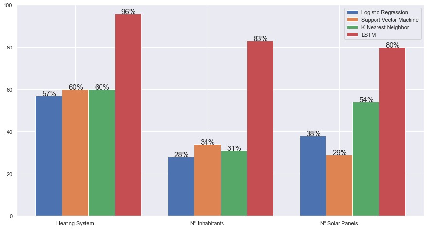
As seen in the bar-chart, the first three models have a relatively low accuracy compared to the results of the LSTM.
The machine learning algorithms LR, SVM and KNN cannot give higher accuracy than 60% on the training set to classify the characteristics. This is because LR can only look at one layer of patterns, SVM has limited predictions on big datasets and KNN looks at only one row at a time. The LSTM works with internal memory, which makes the deep learning process possible. The LSTM can classify multiple rows as a pattern, rather than classifying a single row.
In order to completely validate the performs of the machine learning models, all the mentioned evaluation metrics need to be taken into account as to see what percentage of the classification are relevant and who many of them are correctly classified as well.
When comparing the recall and precision of the models, the results indicate that the LSTM model outperforms every other models. The LSTM model had a recall and precision of 96% when predicting the heating system type, whereas the LR was the lowest performing model with a recall and precision of 28% and 23% when predicting the number of inhabitants. As an example, by taking the LSTM for classifying the heating system installed in a dwelling, the model can surmise that 96% of the time predictions are correctly made, 97% of the time the recommended heating system is correctly classified, and 96% of the time the selected heating system is recommended for this dwelling. A summary of the classification metrics is shown in Table 1.
Summary of classification metrics
|
Algorithm |
Predicted Target |
Accuracy |
Recall |
Precision |
|
Logistic Regression |
Heating system |
57% |
57% |
47% |
|
Logistic Regression |
Number of solar panels |
38% |
38% |
33% |
|
Logistic Regression |
Number of inhabitants |
28% |
28% |
23% |
|
K-Nearest Neighbors |
Heating system |
60% |
62% |
61% |
|
K-Nearest Neighbors |
Number of solar panels |
54% |
54% |
54% |
|
K-Nearest Neighbors |
Number of inhabitants |
31% |
32% |
29% |
|
SVM |
Heating system |
60% |
60% |
59% |
|
SVM |
Number of solar panels |
29% |
29% |
26% |
|
SVM |
Number of inhabitants |
34% |
36% |
33% |
|
LSTM |
Heating system |
96% |
97% |
96% |
|
LSTM |
Number of solar panels |
83% |
82% |
83% |
|
LSTM |
Number of inhabitants |
80% |
81% |
79% |
The machine learning algorithms Logistic Regression (LR), Support Vector Machine (SVM) and K-Nearest Neighbor (KNN) perform significantly deficient than Long Short-Term Memory (LSTM). The main reason for this is that LR, SVM and KNN only look at one row of data, which means they can only classify the data per row. This suggest that every row of 15-minute data is classified individually. The assumptions are that the models will not be able to classify the data based on individual 15-minute data rows accurately, because this data provides an insignificant amount of information.
On the other hand, LSTM uses 92 rows of 15-minute data. This provides the model a comprehensive look at the data, which allows the model to classify the data significantly more accurate than the other models. LSTM uses long time series data memorization in order to classify the data. With this data, the LSTM classifies 92 rows as a pattern instead of classifying a single row.
During the research, several approaches were made to improve the results on LR, SVM and KNN. Especially by looking at aggregating the data in daily and weekly resolutions. This allows the models to classify the data more accurately, because it is easier to differentiate data on daily or weekly resolutions instead of 15-minute data. For instance, the energy use on a winter day/week will probably be significantly higher than on a summer day/week. For SVM in special, it is mandatory to aggregate the data, because SVM does not support big datasets. This conveys that working with 15-minute dataset is to substantial to work efficiently with.
After the first iteration of implementing the RNN, the model classified the data with only one row of data which did not show promising results. The input data was then reshaped in order for the data to contain 92 rows of aggregated data, which showed significantly better results than before after a number of iteration. However, these results were not satisfying yet. In order to get better results, the architecture of the LSTM was changed to a simpler model, by removing one hidden layer and removing the dropouts. As a result, the model is significantly improved, where the model classifies the heating systems with 95% accuracy, the number of inhabitants with 80% accuracy and the number of solar panels with 75% accuracy. Furthermore, the loss function was then changed multiple times for each possible classification. To classify the number of inhabitants better, the loss function “Binary Cross-Entropy Loss” was used and for the number of solar panels, the loss function “Categorical Cross-Entropy Loss" was used. This concludes into the results mentioned in the previous chapter.
The LSTM performs best when it comes to classifying the type of heating system. The number of inhabitants is difficult to classify, since every inhabitant has their own energy use pattern and hours spend in the dwelling, as well as the types of devices they use. For instance, a single inhabitant can spend as much energy in a week as a family of three. The number of solar panels can also be quite more difficult to classify, because smart meter data only provides the produced energy subtracting the used energy in the dwelling.
This paper compares several machine learning algorithms to classify 33 different dwellings from a neighbourhood called Groene Mient based on the following characteristics: heating system type installed, number of inhabitants and number of solar panels installed. Classifications were done with a daily resolution for Logistic Regression and Support Vector Machine and weekly resolution for K-Nearest Neighbors. For the LSTM, 15-minute resolutions were used to feed the model with samples of 92 rows (1 day), by using the energy delivery, consumption, KNMI data and several dummy variables as features. As it is a classification problem, the models have been applied in the following order: Logistic Regression, Support Vector Machine, K-Nearest Neighbors and Long Short-Term Memory.
LSTM performed best compared to the other algorithms for all the target variables (96% on predicting heating systems, 83% on predicting number of inhabitants and 80% on predicting number of solar panels). Based on these results, it has been proved that different dwelling characteristics can be accurately predicted with the use of machine learning algorithms, in specific recurrent neural networks. These results can be used for policy-making decisions regarding the NZEB-standard from government-organisations. This is done by classifying the installed type of heating system, the number of solar panels, and the number of inhabitants.
Behavioural patterns of inhabitants have formed the characteristics of dwellings and their effect on the electricity consumption. This has led to how certain characteristics of dwellings can be controlled to reduce the electricity consumption. As a result, the reasoning for the need of gaining more insight in these dwelling characteristics by using for instance machine learning algorithms is needed, as it has been proved that these algorithms can provide accurate answer to certain questions.
Limitations of this research are that the provided dataset contained missing values, causing an unexplainable gap for certain periods of time. Also, 15% of the dwellings were removed due to the fact that they contained missing values. Furthermore, multiple important dwelling characteristics were not shared due to confidentiality reasons, which limits the explainability and performance of the created models.
Further studies should focus on exploring the possibilities of getting more insight from dwellings by using datasets with a smaller time interval. This allows the LSTM model to possibly perform better. With the purpose of improving the evaluation metrics, it would also be possible by using more sample dwellings and resampling the actual data, which magnify the dataset. This is substantiated on the variance between the validation and train loss of each algorithm. Improving the smart meters collecting method (preventing outliers and blank gaps) will help with the recognition of human patterns and dependencies on outside weather conditions. Alongside this, more features of the dwellings can be used to improve the accuracy of all the algorithms.
- Energy Agenda: towards a low-carbon energy supply , 2017
- Energy in the Netherlands 2019, 2020, www.energieinnederland.nl
- , Sustainable Systems Implementation Building a Sustainable Economy and Society, CSRwire.com, 2007
- ,
Sustainability Assessment in Housing Building Organizations for the Design of Strategies against Climate Change ,HighTech and Innovation Journal , Vol. 1 (4),pp 136-147 , 2020, https://doi.org/10.28991/HIJ-2020-01-04-01 - ,
A Nearly Net-Zero Exergy District as a Model for Smarter Energy Systems in the Context of Urban Metabolism ,Journal of Sustainable Development of Energy, Water and Environment Systems , Vol. 5 (1),pp 101-126 , 2017 - ,
Architectural Rehabilitation and Sustainability of Green Buildings in Historic Preservation ,HighTech and Innovation Journal , Vol. 1 (4),pp 172-178 , 2020, https://doi.org/10.28991/HIJ-2020-01-04-04 - ,
Defining nearly zero-energy housing in Belgium and the Netherlands ,Energy Efficiency , Vol. 5 (3),pp 411-431 , 2012, https://doi.org/10.1007/s12053-011-9138-2 - ,
Potential of Demand Side Management to Reduce Carbon Dioxide Emissions Associated with the Operation of Heat Pumps ,Journal of Sustainable Development of Energy, Water and Environment Systems , Vol. 1 (2),pp 94-108 , 2013 - ,
Smart metering in the Netherlands: What, how, and why ,International Journal of Electrical Power & Energy Systems , Vol. 109 ,pp 719-725 , 2019, https://doi.org/10.1016/j.ijepes.2019.01.001 - ,
Smart meter data: Balancing consumer privacy concerns with legitimate applications ,Energy Policy , Vol. 41 ,pp 807-814 , 2012, https://doi.org/10.1016/j.enpol.2011.11.049 - ,
Green Envelop Impact on Reducing Air Temperature and Enhancing Outdoor Thermal Comfort in Arid Climates ,Civil Engineering Journal , Vol. 5 (5),pp 1124-1135 , 2019, https://doi.org/10.28991/cej-2019-03091317 - ,
Household electricity consumption and CO2 emissions in the Netherlands: A model-based analysis ,Energy and Buildings , Vol. 86 ,pp 403-414 , 2015, https://doi.org/10.1016/j.enbuild.2014.09.077 - ,
Behavioral patterns and profiles of electricity consumption in dutch dwellings ,Energy and Buildings , Vol. 150 ,pp 339-352 , 2017, https://doi.org/10.1016/j.enbuild.2017.06.015 - ,
The smart meter and a smarter consumer: quantifying the benefits of smart meter implementation in the United States ,Chemistry Central Journal , Vol. 6 (1),pp S5 , 2012, https://doi.org/10.1186/1752-153X-6-S1-S5 - , Smart meter data analysis, PES T D 2012, 2012
- ,
Smart meters and household electricity consumption: A case study in Ireland ,Energy & Environment , Vol. 29 (1),pp 131-146 , 2018, https://doi.org/10.1177/0958305X17741385 - ,
Forecasting residential gas consumption with machine learning algorithms on weather data ,E3S Web of Conferences , Vol. 111 ,pp 05019 , 2019, https://doi.org/10.1051/e3sconf/201911105019 - Daily weather data in the Netherlands, www.knmi.nl/nederland-nu/klimatologie/daggegevens
- ,
A deep learning framework for building energy consumption forecast ,Renewable and Sustainable Energy Reviews , Vol. 137 ,pp 110591 , 2021, https://doi.org/10.1016/j.rser.2020.110591 - ,
Big Data Analytics for Discovering Electricity Consumption Patterns in Smart Cities ,Energies , Vol. 11 (3),pp 683 , 2018, https://doi.org/10.3390/en11030683 - , Machine Learning for Sequential Data: A Review, Structural, Syntactic, and Statistical Pattern Recognition, 2002
- ,
Resource and Energy Saving Neural Network-Based Control Approach for Continuous Carbon Steel Pickling Process ,Journal of Sustainable Development of Energy, Water and Environment Systems , Vol. 7 (2),pp 275-292 , 2019 - , , Machine Learning in Radiation Oncology, 2015
- ,
The Influence of the Activation Function in a Convolution Neural Network Model of Facial Expression Recognition ,Applied Sciences , Vol. 10 (5),pp 1897 , 2020, https://doi.org/10.3390/app10051897 - , An Empirical Study of Distance Metrics for k-Nearest Neighbor Algorithm, The 3rd International Conference on Industrial Application Engineering 2015 (ICIAE2015), 2015
- , Applying LSTM to Time Series Predictable through Time-Window Approaches, Artificial Neural Networks — ICANN 2001, 2001
- ,
Improving Electric Energy Consumption Prediction Using CNN and Bi-LSTM ,Applied Sciences , Vol. 9 (20),pp 4237 , 2019, https://doi.org/10.3390/app9204237 - , Understanding dropout, Proceedings of the 26th International Conference on Neural Information Processing Systems - Volume 2, 2013
- , Construction Model Using Machine Learning Techniques for the Prediction of Rice Produce for Farmers, 2018 IEEE 3rd International Conference on Image, Vision and Computing (ICIVC), 2018