


Mangroves are essential environmental ingredients, ensuring the stability of the coastal area. They continue to provide protection against natural and adverse phenomena. They function as a vast sink for carbon sequestration and storage, ensuring sustainability. These wetland vegetations are also important for socio-economic development. Despite mangroves providing shelter and being a source of raw materials for the consumption of humans and other aquatic habitats, they have shown vulnerability against some climatic factors and Land Use Land Cover (LULC) changes [1]. Mangroves continue to get threatened by the rapid development of coastal areas (e.g., aquaculture, industries, etc.) and direct wastewater discharge into the ocean containing fertilisers, heavy metals, microplastics, etc., further contributing to the inertia in their growth [2]. Despite mangroves decreasing globally, many developed countries, including United Arab Emirates (UAE), are keen to conserve these natural resources by employing plantation and public awareness to revitalise their status [3].
One study investigated the response of different mangrove species to chilly weather temperatures [4]. Results indicated that the damaging effects of winter temperature substantially varied per geographic location and mangrove species. Also, foreign mangrove species were less tolerant to low temperatures than native mangroves. Another study investigated the expansion and contraction of mangroves in the wetland of the Mississippi River (Louisiana, USA) [5]. Historical air temperature data (1983-2014) and coastal wetland coverage data (1978-2011) were gathered to identify the connection between climate and mangrove changes. Mangrove trees’ density was found to be controlled by extreme air temperatures below -6.3 to -7.6 °C. Mangroves that were located near oceans were protected against low temperatures due to the presence of water and saturated soil. The frequent occurrence and intensity of freezing events governed the expansion and contraction of freeze-sensitive mangroves in coastal areas. Lovelock et al. reviewed the effects of climate change on mangrove forests [6]. This study showed that low temperatures can deter mangrove growth and influence its metabolic process of photosynthesis and respiration. Another study provided a global analysis of mangrove canopy height based on temperature and other factors [7]. Multivariate regression analysis showed that the mean temperature of a mangrove forest could explain 74% of the latitudinal trends in maximum mangrove canopy height. The model’s results were used to evaluate the impact of temperature on the spatial variability of mangroves. This finding was consistent with previous studies that have shown mangrove structures (i.e., height and biomass) are influenced by temperature. Further analysis revealed that temperature had explained 53% of the global mangrove canopy height trend. Another study showed that climatic factors are associated with decreasing mangrove species composition and evolution. Furthermore, mangroves’ composition can be influenced by winter temperature based on regression and ANOVA analyses [8].
Salinity can potentially influence other environmental parameters governing the growth of mangroves [9]. For one study, an estimation of the change in salinity with biomass of a stenoecious mangrove species (Heritiera fomes) was conducted by correlating with the dataset from 2004 to 2015. Results indicated that biomass for the mangrove species was higher due to lower salinity levels and vice versa. Carbon stock in the Sundarbans mangrove forest’s above and below ground was assessed by considering different vegetation types and salinity zones [10]. Freshwater zones depicted the highest carbon stock (336.09 ± 14.74 Mg C/ha), followed by moderate and strong salinity zones. However, salinity enhanced the below-ground carbon stock capacity: 57.2% below-ground carbon stock was found in the freshwater zone, whereas 71.9% below-ground carbon stock was found in a strong salinity zone. Another extensive research in the same coastal zone was carried out to evaluate mangrove species distribution based on salinity level at the Sundarban forest [11]. Different mangrove species were found in different salinity zones across Sundarbans and possessed different tolerance levels to changes in salinity. It was concluded that the spatial distribution of the indicator species under the research could contribute to the knowledge of mangrove adaptive nature and variations of plants obtained in areas with different salinity levels. Another study assessed mangrove species’ growth under varying salinity degrees. In high-salinity environments, mangrove seedlings exhibited very low survival rates and other physical characteristics. Alternatively, low salinity promoted promising growth of the mangrove plants for 4-5 months. However, further growth and sustenance were observed when the plants were introduced to low to moderate salinity treatment after 15-20 weeks. This research provided an important insight into mangroves’ requirement for varying degrees of salinity, achieving their fullest development [12].
Mangrove expansion can be hindered by the effects of tidal inundation [13]. Rapid propagation of mangroves was possible when water level and wind speed were reduced. It was concluded that interactions between mangrove growth and external drivers (i.e., tidal waves, erosion, etc.) were important to protect the aquatic plant species at such events. Another study analysed intertidal wetland areas and mangrove proportions [14]. Numerous intertidal regimes at 184 NSW (New South Wales) estuaries were investigated, obtaining different combinations of average frequency, duration, and depth of inundation. It was observed that estuary proportion, morphology and entrance condition influenced the tidal aspect inside it. Concurrently, the specifications mentioned above of estuary governed the proportion of mangroves.
Satellite images can be useful in understanding the factors affecting the mangrove growth pattern. A previous study utilised Landsat imageries throughout 1990-2020 to detect the changes in Land Use Land Cover (LULC) and mangrove wetlands [15]. Noticeable LULC alteration was detected over the period. Primarily, aquaculture increased concerning the reduction in agriculture, and this phenomenon was further validated by the Normalised Difference Vegetation Index (NDVI) and Normalised Difference Water Index (NDWI). It was also stressed that the shift in human preference towards aquaculture negatively affected the mangrove ecosystem, and appropriate measures should be taken to preserve mangrove forests. A similar study was done on the LULC change with Land Surface Temperature (LST) and NDVI using Landsat images and found declination in the sizes of mangrove forests from 2000 and onwards [16]. Also, the NDVI values for the mangrove areas were reduced. LST has shown a negative correlation with NDVI for mangroves, indicating that non-vegetated land increased during the study period.
Maryantika and Lin (2017) used multi-temporal Landsat images to assess land use and mangrove distribution for the Sidoarjo district of East Java from 1995-2015 [17]. It was observed that cropland and bare land were repurposed as built-up areas. Conversely, mangrove and other wetland areas changed to cropland resulting from economic activities. A new classification scheme for the northern UAE mangrove forests was used by incorporating Random Forest (RF), Kernel Logistic Regression (KLR), Native Bayes Tree (NBT) and Image Difference (ID) to make accurate mangrove extent monitoring in comparison to traditional classifiers (e.g., maximum likelihood) [3]. Also, RF, KLR, NBT and ID algorithms were evaluated based on their performance and an image-to-image change detection technique to monitor mangroves in the northern UAE was developed.
GIS and Remote Sensing techniques were used in several other applications. One investigation assessed the temporal status of Buyuk Melen Watershed using Landsat images collected for 1987, 2001, 2006 and 2010. LULC changes were detected in the study area, along with increased water pollution [18]. Another endeavour used Random Forest (RF) algorithm to map soil moisture content for irrigation purposes. RF was also pitted against the neural network model and turned out superior for this work [19]. A study was conducted on the glacier surface of Ampay National Sanctuary using historical Landsat images. Supervised classification with normalised snow differential index applied on the satellite images revealed that glacier surface decreased yearly with the variations of climatic factors, e.g., increasing temperature [20]. Tidal inundation affected mangroves in an unfavourable way [13]. LULC classification of mangroves over a specified duration indicated a general fall in mangrove sites to be replaced with croplands or other built-up areas [17].
After numerous literature reviews, it was observed that most previous studies investigated the effect(s) of different environmental and anthropogenic parameters influencing mangrove vegetation health. Still, their evaluation methods were chiefly based on visual interpretation and linear regression. Also, the research mostly considered the effects of the stated parameters individually but did not consider their combined influence on mangrove NDVI. The novelties of this spatiotemporal investigation lay in the fact that it not only covered the impact of LST and salinity on mangrove NDVI separately but also considered their combined influence on mangrove systems by incorporating different levels of analysis arising out of remote sensing and GIS. Furthermore, this research attempted to quantitatively correlate LST and salinity with mangrove vegetation health (i.e., NDVI) to observe the best relationship in terms of various machine learning algorithms (in addition to linear regression) to generate a model to potentially predict future changes of mangrove biomass as a response variable against the predictors (i.e., LST and salinity). Additionally, this scholarly work attempted to identify special patterns, highlighting the relationship between LST-NDVI and salinity-NDVI to look for potential range in the explanatory variables that might provide high mangrove biomass under the study area.
To achieve the objectives, the authors describe the location of the mangrove ecosystem in the UAE. The section describes satellite image collection, processing and the methodologies for developing correlation with different relevant parameters.
UAE mangrove sites
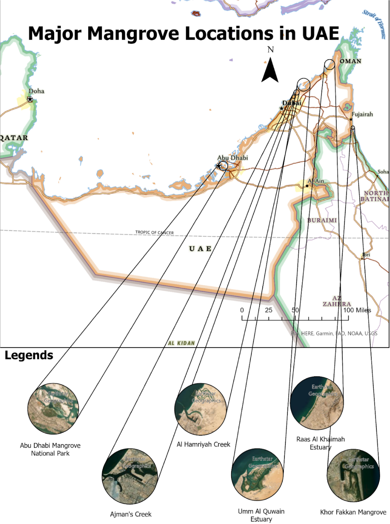
There are eleven major mangrove forests in the UAE. Essentially, the UAE mangrove ecosystem was broadly divided into two sectors. One resided in Abu Dhabi, and the other in Northern UAE. The Abu Dhabi Forest covered 70 km2, with the primary forest being the Mangrove National Park which spanned about one-third of the total forest area [21]. The Northern UAE mangrove forests were distributed in six areas, including Dubai’s Creek, Khor Fakkan mangrove (Gulf of Oman), Ajman’s Creek, Hamriyah’s Creek, Umm Al Quwain and Ras Al Khaimah (RAK) Estuaries. The average UAE mangrove trees’ height was about 2.5 m [22]. The dominant soils in these areas were porous loamy silt and clay with relatively low permeability. These characteristics allow the retaining of seawater within the soil structure [23]. Figure 1 shows the locations of the UAE mangrove forests.
Landsat Images were used to study the UAE mangrove forests in 2004, 2010, 2015 and 2020. The image acquisition periods were consistent with reducing atmospheric interference effects when analysing the relevant parameters to assess mangrove conditions influenced by external events. For this study, images were obtained for the summertime (e.g., between June and July) with less than 10% cloud cover. Landsat satellite images were primarily chosen because of their suitable resolutions and availability of spectral bands to detect and represent topographic changes in response to environmental and anthropogenic parameters. Also, these images were freely acquired.
Landsat 7 satellite images were obtained for 2004 and 2010. Finally, Landsat 8 satellite covered the periods 2015 and 2020. Landsat 7 had an Enhanced Thematic Mapper (ETM+). Landsat 8 carried Operational Land Imager (OLI) and Thermal Infrared Sensors (TIRS) devices. Red and Near Infrared (NIR) bands were used for each Landsat satellite to compute NDVI, and a thermal band was used to detect LST. Salinity data were obtained by searching relevant literature [24] to develop a suitable empirical model with visible and Near Infrared bands’ reflectance values. Salinity was represented as electrical conductivity in units of dS/m.
Landsat images were radiometrically corrected to eliminate atmospheric interference caused by absorption, scattering, etc., of solar radiation by clouds and other airborne particles. The correction enabled extracting refined information from the images to perform accurate quantitative analysis. This process involved the conversion of raw Digital Numbers (DNs) of satellite images to radiance and, ultimately, reflectance. At first, DN values were converted to radiance, defined as the energy flux (i.e., irradiant/incident energy) per solid angle, leaving a unit surface area in a given direction.
(1)
Where: Lλ - spectral radiance at the sensor’s aperture , M_L - band-specific multiplicative rescaling factor from Landsat image metadata file, A_L - band-specific additive rescaling factor from Landsat metadata file, Qcal - quantised and calibrated standard product pixel value (DN).
Then, spectral radiance was converted into Top of Atmosphere (TOA) reflectance:
(2)
Where: ρp - TOA reflectance (ratio of the reflected solar energy to incident solar energy), Lλ - spectral radiance at the sensor’s aperture , d - Earth-Sun distance in astronomical units (provided in the image metadata file), ESUNλ - mean solar exo-atmospheric irradiance , θs - solar zenith angle, i.e., the angle between the sun’s rays and the vertical direction [25].
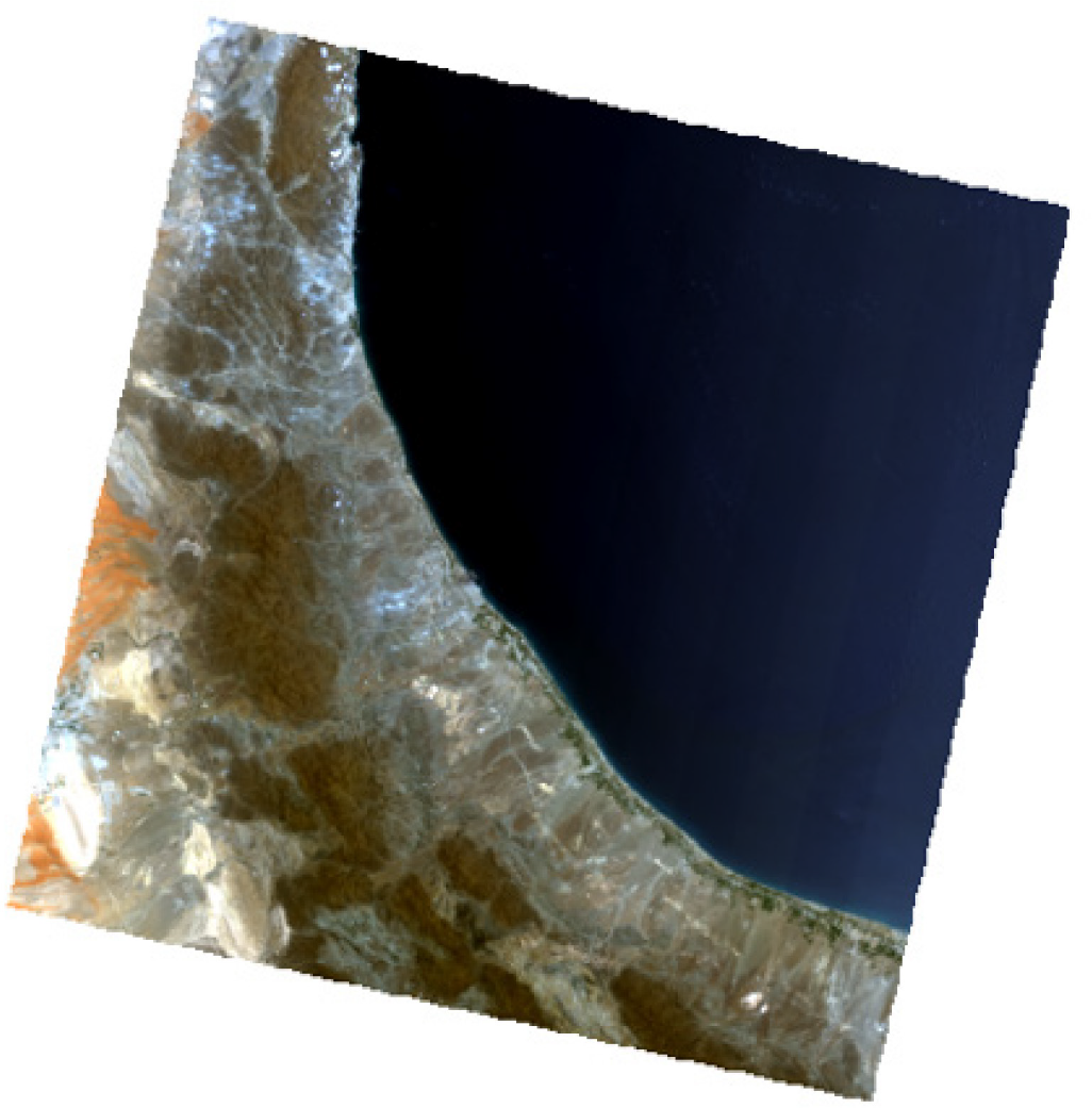
After the preprocessing, Landsat images for each considered year were band stacked in the order of the band numbers so that different band combinations could be applied to the colour gun of the software to effectively visualise and further analyse different features found in the image along with making the images vibrant (Figure 2).
Radiometrically corrected Landsat 8 multi-band raster image of 159 path and 043 row
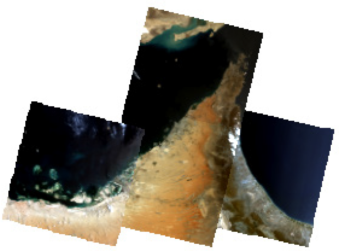
Detailed particulars of the images used for the study are provided in Table 1. All the images were reprojected into a common Projected Coordinate System (PCS), WGS 1984 UTM Zone 40N. The images mentioned below cover the entirety of the UAE. Then, the band stacks for a specific year were mosaicked to form a whole image showcasing UAE mangroves in Figure 3.
Landsat image acquisition particulars
| No. | Satellite name | Acquisition year | Image path and row |
|---|---|---|---|
| 1 | Landsat 7 ETM+ | 2004, 2010 | 159043, 160042, 160043, 161043 |
| 2 | Landsat 8 OLI & TIRS | 2015, 2020 |
NDVI is one of the spectral indices commonly used to signify the health and extent of mangrove vegetation. It is derived from the ratio of several bands found from Landsat satellite(s). NIR and Red bands compute NDVI [26]:
(3)
For Landsat 5 and Land Sate 7 satellite images, bands 3 and 4 were considered visible Red and NIR. For Landsat 8, bands 4 and 5 were Red and NIR respectively.
Mosaic raster bands for UAE in 2020
Thermal band 6 for Landsat 5 and 7 & 10 TIRS 1 for Landsat 8 had at-sensor spectral radiances, which were first converted to effective at-sensor brightness temperatures using the formula:
(4)
Where: T - effective at-sensor brightness temperature, K2 - calibration constant equal to 2 K, K1 - calibration constant equal to 1 , Lλ - spectral radiance at the sensor’s aperture .
The spectral radiance represents energy flux (measured in watts) per unit solid angle (1 steradian), leaving a unit surface area (1 m2) per unit wavelength (1 μm).
Then, the brightness temperature (i.e., the surface temperature in kelvin) was converted into degrees Celsius [26].
For Landsat 8, LST was computed using multiple steps and formulas. It was obtained using band 10 (Thermal Infrared) with 100 m spatial resolution. The top of atmospheric spectral radiance was computed from band 10, followed by the radiance conversion to at-sensor temperature. After that, the NDVI method was applied for emissivity correction. Finally, LST was computed from land surface emissivity [27]. For Landsat 7, the thermal band (i.e., band 6) was found in both low and high gain. The high gain thermal band was used because it was suitable for computing LST for vegetation. Also, for Landsat 8, thermal band 10 was used for LST to avoid large calibration uncertainty in thermal band 11.
Sample locations were chosen within the AOIs covering the mangrove sites in Figure 1 as zones. Each zone consisted of 9 pixels with 30 m by 30 m pixel size, resulting in 90 m by 90 m zone size respectively. A total of 30 zones for the 11 mangrove forests were finalised. These sectors were selected so that each zone covered its representative mangrove biomass and was in proximity to the coastal line so that any localised variation of LST and Salinity would impact the mangrove biomass condition covered by that zone. Zonal statistics of the yearly variations of the parameters could be referred to and documented to examine potential trends.
Salinity throughout the mangrove areas (i.e., 30 zones) was obtained as electrical conductivity by referring to an empirical model proposed by Asfaw et al. (2018) with a coefficient of determination equalling 0.78. The model used the salinity index (SI) [24]. The formulas for soil salinity computation are provided below.
(5)
(6)
After gathering data on NDVI, LST and Salinity extracted from the predefined mangrove zones for the four years, they were first transferred to an Excel sheet for the sequential organization. Then, all the data were imported using MATLAB’s regression learning package to start a new session. Under the features, NDVI for a particular year was selected as a response variable, and LST & Salinity for that year were chosen as predictors. Before the actual model training, a validation scheme was selected by default to understand the predictive accuracy of the viable model and avoid over-fitting. Once all the options were set up, the available data were run for three combinations (NDVI-LST, NDVI-Salinity and NDVI-LST-Salinity). In addition to the basic linear regression function, the MATLAB package simulated the data for other machine learning algorithms such as regression trees, Support Vector Machines (SVMs), Gaussian Process Regression (GPR) and an Ensemble of Trees (details provided in Table 2) by considering all their variations (19 in total).
List of all the employed machine learning algorithms
| No. | Machine learning algorithms | Sub-categories |
|---|---|---|
| 1 | Linear Regression Models | Linear Interaction Linear Robust Linear Stepwise Linear |
| 2 | Regression Trees | Fine Tree Medium Tree Coarse Tree |
| 3 | Support Vector Machines (SVM) | Linear Quadratic Cubic Fine Gaussian Medium Gaussian Coarse Gaussian |
| 4 | Gaussian Process Regression (GPR) | Rational Quadratic Squared Exponential Matern 5/2 Exponential |
| 5 | Ensemble of Trees | Boosted Trees Bagged Trees |
Linear regression models are statistical measures to formulate a relation between two or more variables by incorporating a linear equation into the collected data. Regression trees are decision trees that predict continuous value based on one or more input variables. Support Vector Machines are used for both classification and regression analysis. They achieve this by segregating acquired data into different classes or groups. Gaussian Process Regression is a probabilistic machine learning algorithm that uses the Gaussian process to model the relationship between dependent and independent variables. Ensemble of Trees combines decision trees to form prediction models suitable for analyzing structured data to generate meaningful information.
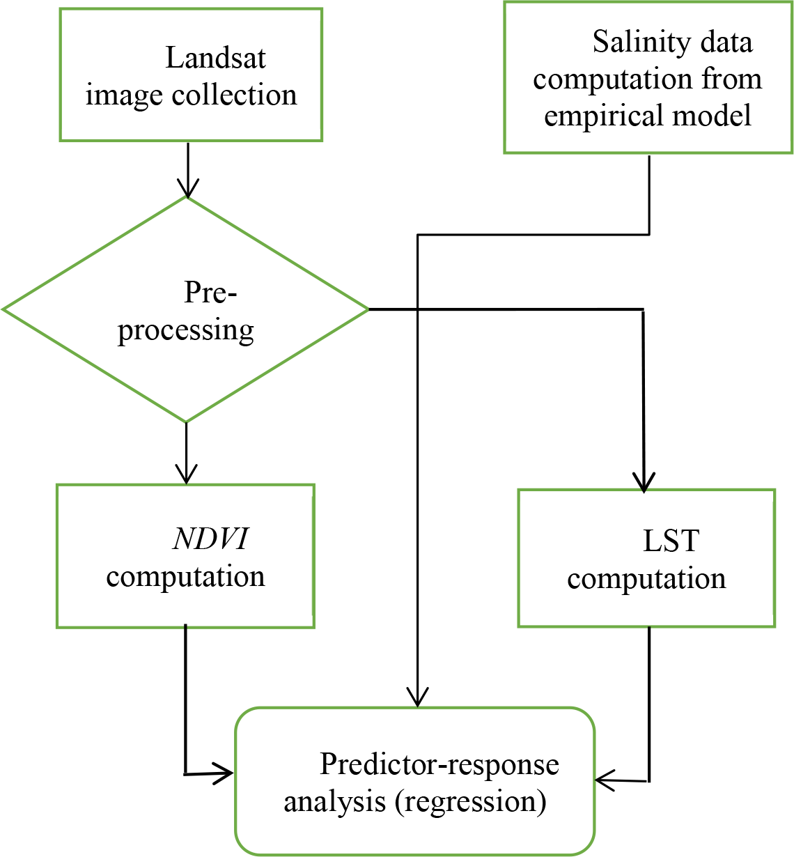
The incorporation of different machine learning algorithms was done because the supposed intricate relationship between mangrove biomass might not fully relate linearly with land surface temperature and coastal salinity, and other feasible associations could exist. After running and completing all the instruction sets simultaneously, the best output was chosen for each of the three relationship types based on the lowest RMSE and highest R2. Then, response plots were visualised to observe the models for potential patterns regarding the arrangements of true data points and the resulting predictive trends with the variations of the dependent and independent features. The finalised models could be further optimised for better predictions by implementing feature ranking algorithms. But it was left out because the order of importance for the predictors could not be settled by exploring the existing scholarly works. Therefore, when a combined assessment was conducted, equal importance was given to both LST and Salinity when assessing mangrove NDVI. Also, an option was available for exporting the feasible models and functions for future fine-tuning by incorporating the representatives with additional data. Figure 4 denotes the chronological procedures for conducting the investigation.
Flow chart for the sequential methods
For all the predefined locations from where NDVI, LST and Salinity values were extracted by employing tabular zonal statistics operation in ArcGIS Pro 3.0, the resulting variables were introduced to several machine learning algorithms, including linear regression, regression trees, SVM, GPR and the ensemble of trees (Table 2) to find out the highest correlations amongst them in terms of lowest RMSE for each year. The process was repeated for four years to cover 2000-2020, validate the relationships further, and assess their consistency. Therefore, the uniqueness of this study is to avail several regression processes to find out the best match between NDVI, LST and Salinity for the mangrove ecosystems from the prediction trends. Also, response plots indicating true and predicted mangrove vegetation health for given LST and Salinity were visually observed to reveal interesting patterns.
Out of all the suitable regression models between LST and NDVI, Support Vector Machine (SVM) with a Medium Gaussian kernel demonstrated the best relationship between the two parameters for 2010 with a minimum RMSE value of 0.0368 and maximum R2 value of 0.330 (Table 3). Other attempted regressions, for 2004 and 2020, generated unsatisfactory outcomes with no correlation between mangrove biomass with land surface temperature variation.
Most suitable models to relate NDVI with LST for each year
| No. | Year | Regression model | RMSE | R2 |
|---|---|---|---|---|
| 1 | 2004 | Support Vector Machine (SVM Cubic) | 0.099 | 0.060 |
| 2 | 2010 | SVM (Medium Gaussian) | 0.067 | 0.330 |
| 3 | 2015 | SVM (Medium Gaussian) | 0.076 | 0.300 |
| 4 | 2020 | Ensemble (Bagged Trees) | 0.111 | 0.010 |
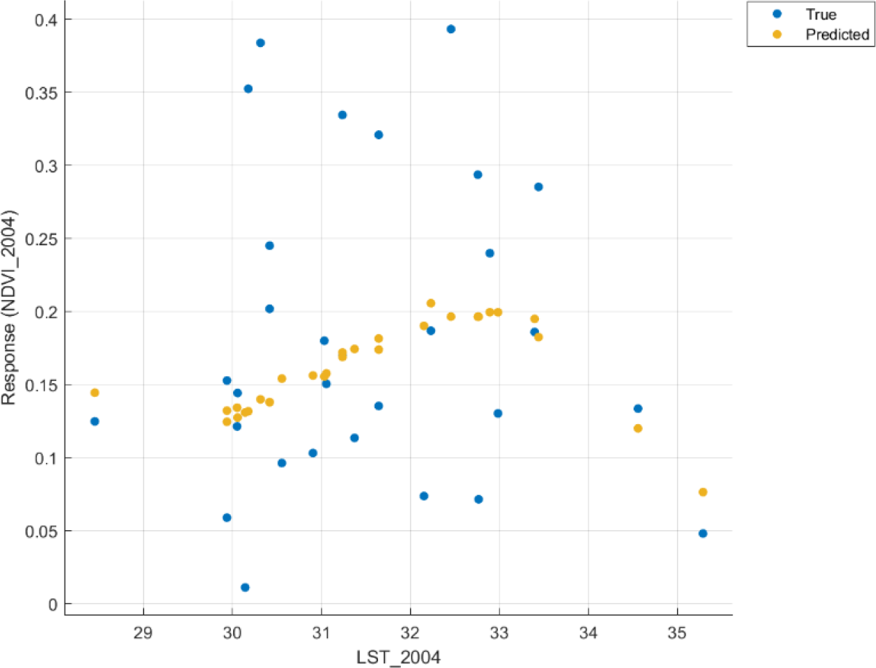
From Figures 5 to 8, it was found that the true data points were mostly scattered with no definitive pattern to assess the predictability. By considering yearly predicted mangrove NDVI variations against the LST, predicted mangrove biomass grew from 2004 by around 0.10 to 0.15, indicating improved health for mangrove plants residing in the chosen zones. It seemed mangroves flourished at a specific temperature range, and extreme temperatures could negatively affect vegetation health. For 2004 (Figure 5), predicted points showed an increase in NDVI from 0.13 to a maximum of 0.20, occurring with an increase in temperature from 30 to 33 °C. Progressing from that upper limit for LST meant less mangrove biomass.
Normalised Difference Vegetation Index (NDVI) as a function of Land Surface Temperature (LST) for 2004
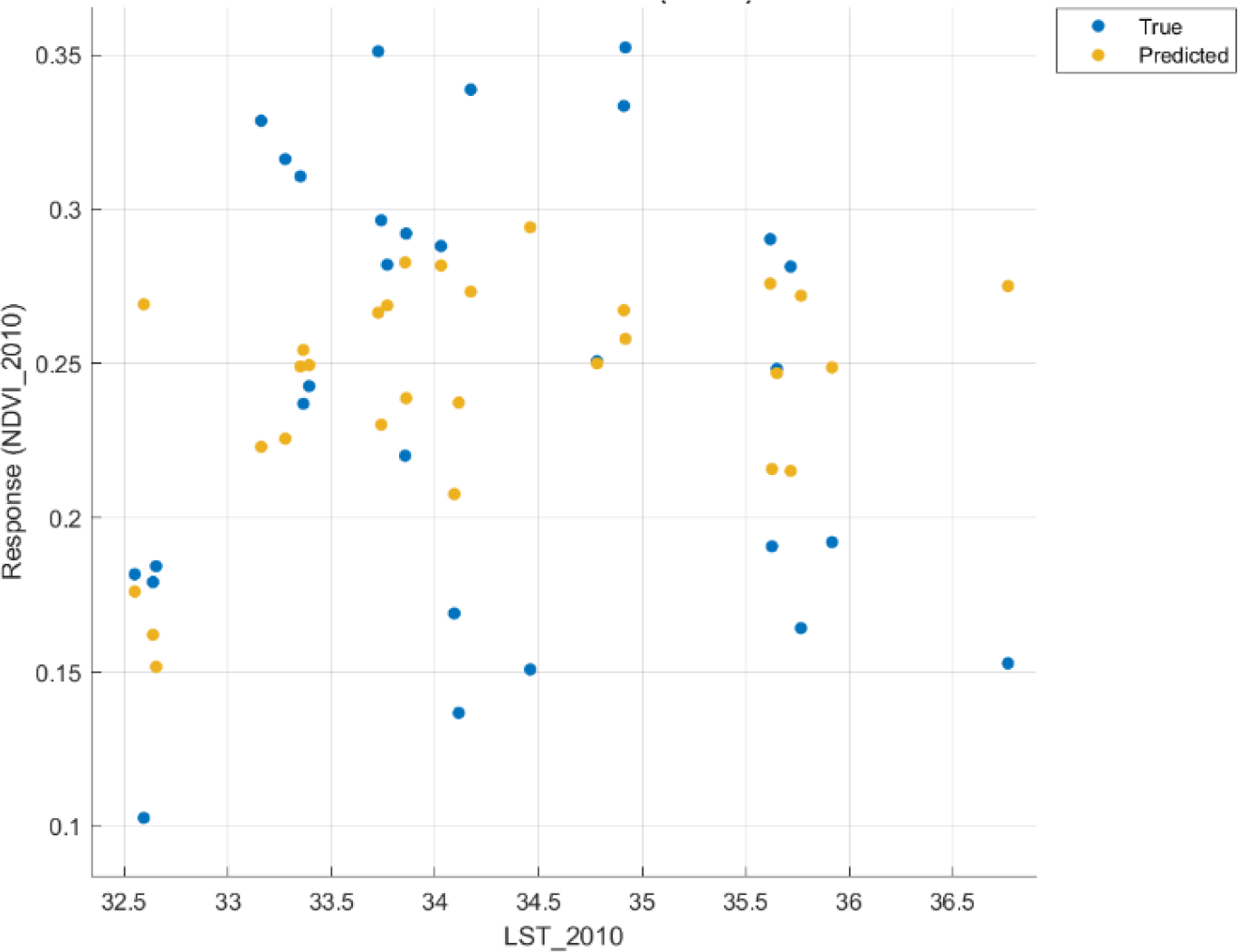
For 2010, observed data points highlighting mangrove biomass response to surface temperature were vastly scattered to delineate any noticeable pattern. The disorganization of predictions also supported it. However, upon careful observations, it could be discerned that mangrove NDVI tended to exhibit a reasonable value of around 0.27 at temperatures between 33.5-34.5 °C. Mangrove biomass again exhibited fluctuations in NDVI between 35.5-36 °C (Figure 6).
NDVI vs. LST 2010
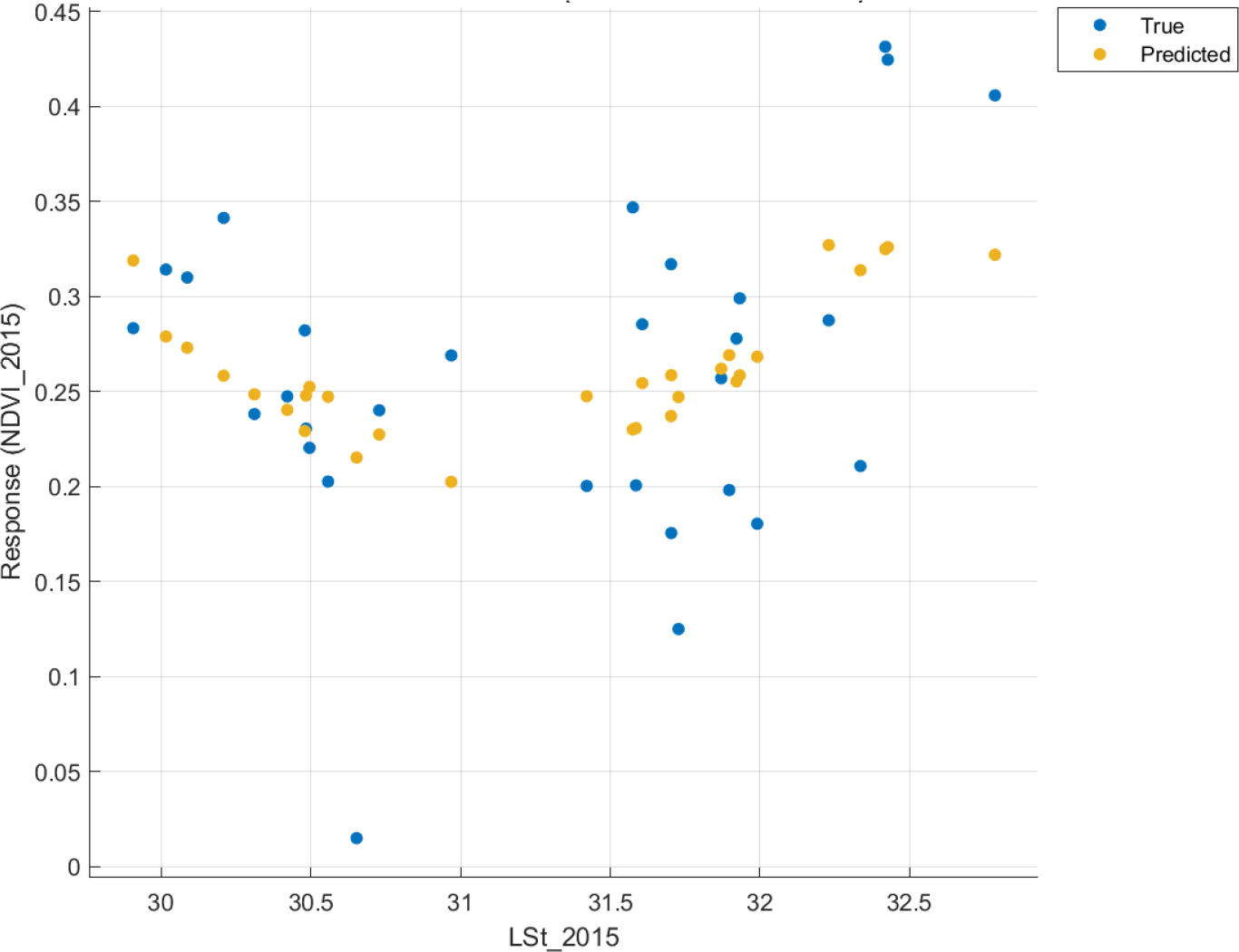
For 2015 (Figure 7), increased LST led to decreased predicted mangrove biomass between 30-31 °C. From 31.5 °C onwards, there was an upshift in mangrove NDVI from 0.22 to a maximum of around 0.33 from approximately 31.5 to 32.5 °C.
NDVI vs. LST 2015
NDVI vs. LST response plots for 2020 did not provide any visually explainable trend. Still, a wide range of mangrove vegetation health was predicted between 31-34 °C as a cluster. Also, neither observed nor predicted vegetation was found in the temperature range from 34.3 to 35.5 °C due to the lack of their influence (Figure 8).
NDVI vs. LST 2020
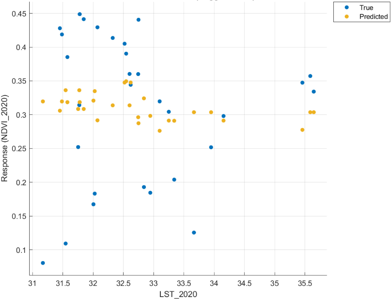
Table 4 shows that for all the years considered, there was a negligible correlation between Salinity and mangrove biomass. But amongst all the regression models, SVM (linear) established a small correlation between Salinity and NDVI with a minimum RMSE of 0.071 and an R2 value of 0.180. For all other cases, severely low R2 values coupled with significantly larger RMSEs rendered them invalid at explaining a general trend.
Most suitable models to relate NDVI with LST for each year
| No. | Year | Regression Model | RMSE | R2 |
|---|---|---|---|---|
| 1 | 2004 | Tree (Medium) | 0.10732 | 0.02 |
| 2 | 2010 | SVM (Linear) | 0.070589 | 0.18 |
| 3 | 2015 | Tree (Medium) | 0.083912 | 0.05 |
| 4 | 2020 | SVM (Fine Gaussian) | 0.11021 | 0.03 |
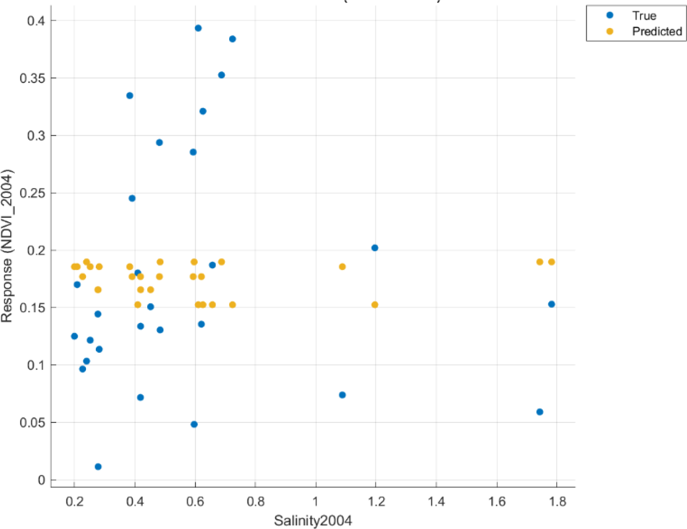
Like with NDVI-LST variations, response curves for NDVI-Salinity (Figures 9 to 12) did not project a particular pattern in the distribution of true values. However, Figure 10 shows a steady fall in predicted mangrove NDVI with increasing Salinity observed for 2010. Also, at lower Salinity values, there seemed to be some high true NDVI values for mangrove sites for all the chosen years. Unfortunately, no valid predictions could be made to propose a trend in the relationship between Salinity and the corresponding mangrove biomass for 2004 (Figure 9), 2015 (Figure 11), and 2020 (Figure 12) solely based on the coefficient of determination and root mean square error. However, closer inspection to identify patterns in the behaviour of predicted mangrove biomass in response to changing Salinity revealed that for 2004, mangrove biomass varied between 0.15 and 0.18 for a Salinity range between 0.2 and 0.7. Beyond the threshold of 0.7, no mangrove vegetation health status was confirmed in Figure 9.
Normalised Difference Vegetation Index (NDVI) as a function of Salinity for 2004
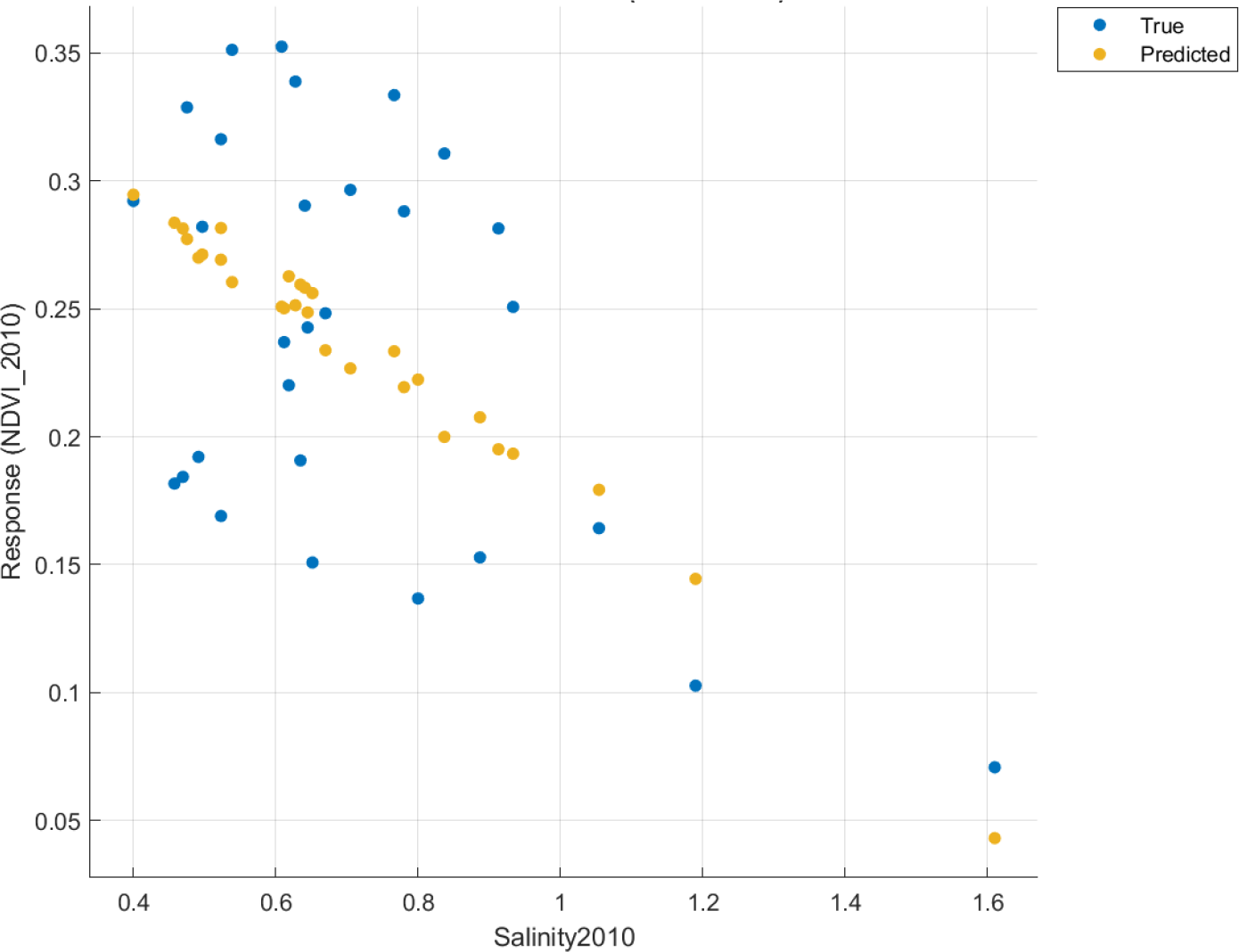
As discussed earlier, there seemed to be a noticeable relationship between coastal salinity and mangrove vegetation health. SVM (linear) predicted that a proportional decrease in NDVI accompanied the increase in Salinity. Furthermore, this pattern was obvious for a Salinity range from 0.4 to 1.2. Beyond this range, mangrove biomass was absent in Figure 10.
NDVI vs. Salinity 2010
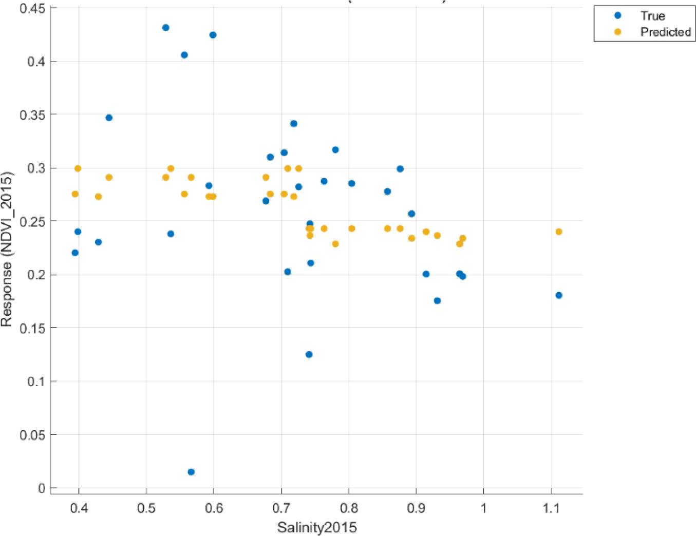
2015 divulged a not-so-distinctive order to model NDVI-Salinity variation compared to 2010 (Figure 10). Still, there seemed to be average predictive mangrove vegetation with NDVI of about 0.28 as a response to the Salinity range from 0.4 to 0.7. A further increase in Salinity from 0.75 to 0.98 rendered a slight decrease in mangrove vegetation with an NDVI of around 0.24 (decreased by 0.04) in Figure 11.
NDVI vs. Salinity 2015
When considering 2020, a diverse range of predicted mangrove vegetation health was observed as a cluster between Salinity values of 0.2 and 0.75. The maximum predicted NDVI for the cluster was found to be around 0.45, and a minimum NDVI value was seen to be at 0.24, with an average of around 0.33. Coastal salinity for the selected sites did not exceed 0.75 in most cases to yield any value for the mangrove biomass beyond that threshold in Figure 12.
NDVI vs. Salinity 2020
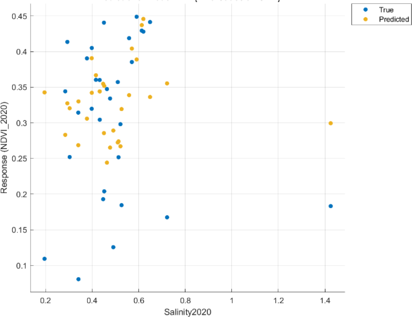
Table 5 demonstrates the combined effects of LST and Salinity on mangrove NDVI. For all the years considered, it seems there was a relatively more significant combined influence by the predictors on the response variable than their contribution to altering NDVI dependency on them. Gaussian Process Regression (Squared Exponential) showed the best possible correlation between NDVI and LST, and Salinity for 2020. SVM (Quadratic) came in second best. However, the Tree (Coarse) model failed to generate any such relationship for multi-regression analysis.
Most suitable models to determine NDVI against the combined influence of LST and Salinity
| No. | Year | Regression Model | RMSE | R2 |
|---|---|---|---|---|
| 1 | 2004 | SVM (Medium Gaussian) | 0.010 | 0.100 |
| 2 | 2010 | Tree (Coarse) | 0.080 | 0.000 |
| 3 | 2015 | SVM (Quadratic) | 0.076 | 0.280 |
| 4 | 2020 | Gaussian Process Regression (Squared Exponential) | 0.094 | 0.310 |
A joint assessment of the results suggests that mangrove vegetation health flourished at a certain temperature window (i.e., between 30-33 °C). For 2004, between these optimal temperature ranges, mangrove biomass increased from 0.13 to 0.20. In another instance, the LST increase from 29 to 30 °C resulted in the fall of mangrove vegetation health from 0.28 to 0.20. However, between 31.5-32.5 °C, mangrove biomass again showed improvement, increasing NDVI from 0.24 to 0.33. It further confirmed the optimal temperature range in the mangrove systems for their sustenance. Previous research works only assessed the response of mangroves under extreme temperatures [5], [6], [28], but this finding added a new perspective on mangroves, showing development between certain LST values. As for the mangroves’ predictive response to the change in Salinity, vegetation health seemed to deteriorate in response to the increase in Salinity, and this pattern was noteworthy between 2010 and 2015. This finding was also validated by previous studies [9]. Also, compared to 2010, the decrease in mangrove NDVI was less prominent in 2015, exhibiting mangroves’ adaptive nature to increased Salinity. In the end, considering both LST and Salinity to impact mangrove vegetation garnered more influence than the individual factors alone, as indicated by an overall high R2 value (e.g., 0.31).
The limitation of this research was due to the not being able to find out satisfactory R2 and RMSE values by employing different machine learning algorithms when considering NDVI-LST (Table 3), NDVI-Salinity (Table 4) & the combined effects of LST and Salinity on mangrove biomass (Table 5). It largely contributed to the amount and the quality of data employed. More data points might have led to increased accuracy, but it would have required many computations along with time. Also, some models performed better than the rest because of the assumptions they made in predicting the response variable against the observed values by using the corresponding explanatory variables. When the supplied information aligned with the assumption made by a specific mathematical instruction, a viable model was only generated at that instance. As raw data might not be suitable for direct machine learning assessment, the models could be further refined by preprocessing the collected data.
Furthermore, identifying the combined effects of some other parameters along with LST and Salinity (e.g., sea-level rise, tidal inundation, LULC, etc.) on mangrove NDVI would greatly improve the prediction. Additionally, the temperature range proposed for this study is suitable for UAE. Future works by considering mangroves located in different regions worldwide could unveil different LST ranges.
In this study, climate change impacts on mangroves were examined. It was done considering LST as the main climate factor along with the salinity of the coastal water at the mangrove forest locations. Mangrove forest change was represented using the NDVI layers, which were extracted from Landsat imagery along with LST at the forests’ locations and salinity of coastal water. Analysis was carried out to determine the impact of each factor on mangroves and then the combined effect of LST and Salinity on mangroves. The best-fit model, which combines the impact of LST and Salinity on mangroves, was obtained using Gaussian Process Regression (Squared Exponential) with an R2 value of 31.1% and an RMSE of 0.094.
To improve the modelling process in our ongoing efforts to study the impact of these factors on mangroves, higher-resolution satellite imagery will be obtained for recent years. Also, empirical equations for Salinity will be established, which would be particularly catered towards mangrove forests found in the UAE by conducting field visits and taking Salinity measurements at selected locations based on their associations with the existing mangrove forest. Timing will be maintained to ensure that satellite image data are available during field surveys.
The authors would like to acknowledge the support received from FRG21-M-E77 (American University of Sharjah).
| AL | band-specific additive rescaling factor from Landsat metadata file | |
| d | earth-sun distance in astronomical units | |
| ESUNλ | mean solar exo-atmospheric irradiances | |
| K1 | calibration constant 1 | |
| K2 | calibration constant 2 | [K] |
| LST | Land Surface Temperature | [K] |
| Lλ | spectral radiance at sensor’s aperture | |
| ML | band-specific multiplicative rescaling factor from Landsat image metadata file | |
| NDVI | Normalised Difference Vegetation Index | |
| Qcal | quantised and calibrated standard product pixel value | |
| Salinity | soil salinity parameter according to eq. (6) | |
| T | effective at-sensor brightness temperature | [K] |
| Greek letters | ||
| θs | Solar zenith angle in degrees | |
| ρp | TOA reflectance | |
| Abbreviations | ||
| ANOVA | Analysis of Variance | |
| DN | Digital Number | |
| ETM | Enhanced Thematic Mapper | |
| GIS | Geographic Information System | |
| GPR | Gaussian Process Regression | |
| ID | Image Difference | |
| KLR | Kernel Logistic Regression | |
| LULC | Land Use/Land Cover | |
| MATLAB | Matrix Laboratory | |
| NBT | Native Bayes Tree | |
| NIR | Near Infrared | |
| NSW | New South Wales | |
| OLI | Operational Land Imager | |
| RF | Random Forest | |
| RMSE | Root Mean Square Error | |
| SI | Salinity Index | |
| SVM | Support Vector Machine | |
| TIRS | Thermal Infrared Sensor | |
| TOA | Top of Atmosphere | |
| UAE | United Arab Emirates | |
| USA | United States of America | |
| UTM | Universal Transverse Mercator | |
| WGS | World Geodetic System |