Nowadays, climate changes are occurring at a fast pace. According to [1], climate change is estimated to have a significant impact on the water cycle, affecting rainfall patterns and altering underground and surface water availability and quality, agricultural production, and associated ecosystems. It urges that human attitudes change drastically to revert this situation. If nothing is done to overcome this issue, global warming will increase [2]. The temperature will rise, longer and more frequent drought periods, and other extreme weather conditions will occur. Many regions of the world are facing severe water scarcity. Irrigation becomes an important issue. In [3], the authors review the global research in sustainable irrigation in agriculture over the last two decades and the main agents promoting it. These topics have received the most attention. The main concerns are improving irrigation water use, more efficient agriculture (producing more using less water resource), and mitigating the effects of global climate change. Research on sustainable irrigation agriculture is needed to make this technology accessible, as its cost is economically unfeasible for small-scale agriculture in many countries.

Nowadays, decision support systems are widely used in the agricultural sector. They have become indispensable tools to conduct more sustainable and productive agriculture, which is difficult to sustain due to the continuous climate changes [4]. In [5], the authors study how the variation of the climate, climate change, and the siltation of reservoirs will affect land use and how the population growth will challenge the sustainability of engineered river systems in the near future. In [6], the authors present a study on regional climate change impacts on irrigation vulnerable season shifts in agricultural water availability for South Korea. As the authors note, reservoirs are the primary source of irrigation water in South Korea. However, to properly manage reservoirs, it is necessary to know how long are the water shortages. The authors assess the vulnerable seasons of paddy irrigation, enabling more efficient management of the reservoirs. To do so, the authors evaluate the vulnerable seasons taking into account the potential water supply capacity and irrigation water needs, using time series.

In many countries, such as Portugal, most water resources are used to irrigate crop fields. Hence, it is crucial to develop an eficient irrigation plan that can maximize the production of a crop field with the minimum amount of water possible [7]. The report of G20 [1] has as first recommendations to modernize irrigation schemes. It promotes the modernization of large-scale surface irrigation systems to improve irrigation eficiency. The study of irrigation systems and related infrastructure has been previously addressed using Genetic Algorithms. In [8], a model based on on-farm irrigation scheduling and the simple genetic algorithm optimization (GA) method for decision support in irrigation project planning were presented. In [9], a multi-objective fuzzy stochastic model was developed to determine optimum cropping patterns with water balance for the next crop season. In [10], a GA technique was used to evolve an efficient cropping pattern for maximizing benefits for an irrigation project in India. In [11], the authors presented an automatic recommendation irrigation system to minimize water use, where big data analytic techniques have been applied to predict the optimal irrigation. In [12], the authors presented a model to calculate soil moisture based on scarce data. They used soil moisture measurements every two weeks and applied a Random Forests algorithm to estimate daily soil moisture, converting the original data to data with a daily time step; this is very important to any irrigation system where data on soil moisture is scarce. In [13], an optimization model was presented for allocating agricultural irrigation water to improve the efficiency of irrigation water use considering uncertainties of fluctuating water supply. The proposed model's feasibility was demonstrated through its application to an irrigation district in northeastern China. In [14], six irrigation treatments were applied combining different levels of water deficit depending on the phenological stage, and the models AquaCrop and MOPECO were compared with simulations. The authors of [15] presented a review on deficit irrigation management practices minimizing the impact on crop yield (reducing the amount of water provided to the crop during the growing season to a level below that needed for maximum plant growth). They also remarked that attention should be paid towards studying other crops that could withstand irrigation deficit with minimum impact on the yield and quality.

Optimal control theory emerged in the 1950s to solve problems concerning power trains for hybrid vehicles [16] and space exploration of the solar system [17]. It is a recognized tool used in areas such as robotics, biological systems [18], health problems [19], economic problems [20], among many others. The optimal control theory aims to find a control law for a given system to achieve a specific optimality criterion.

This paper proposes to study irrigation systems as an optimal control problem. Previous works by the same authors have shown that the total amount of water spent can be reduced when an irrigation system is modelled as an optimal control problem. In [21] and [22], the solution for a similar problem was numerically validated, taking into account theoretical developments in Optimal Control, namely the Maximum Principle [23]. The analytic solution was obtained and compared with the numerical one. A comparison with a real case was presented to understand the gains of using this approach.

This paper proposes and investigates an improved formulation of an optimal control model, enhancing results previously reported in [21] for obtaining a plan of irrigation of a crop field for a given period. The optimal control model in [21] was formulated to minimize the water used while keeping the crop safe. Horton's equation [24] and the soil water balance model [25] were considered to estimate water losses due to deep infiltration. New features like the soil slope, the possibility to include the percentage of water losses due to runoff, and the percentage of water losses if the soil is at field capacity are added to previous models by the authors.

Moisture sensors in the crop field are used to measure the actual trajectory of the state variable. Considering that several unforeseen events can occur, such as poor performance of the irrigations system or unexpected climatic changes, it is necessary to check if the predicted soil moisture corresponds to the actual humidity. If the correspondence is not verified, corrections must be made by replanning. In [21], a replan strategy was presented considering the precipitation data. However, as it was formulated via penalizing the cost function, it may be difficult to use because the penalization constant is not known a priori. This work proposes a new reformulation of the optimal control problem to overcome this issue. Instead of penalizing the objective function, a new constraint is incorporated to impose that the soil moisture does not violate the state constraint (soil moisture is set with minimum value to guarantee the crop is safe). It requires adding the necessary value to the control variable (the amount of water to irrigate). A new replan algorithm is proposed for obtaining a new irrigation plan based on actual updated values of the soil moisture trajectory.

A new approach to deal with several irrigation points is also proposed. It allows to irrigate rectangular crop fields that may have different crops, different types of soil, and different slopes. The available water can be redistributed if an irrigation point cannot provide all water needed according to the irrigation plan. This is an important step towards obtaining a more realistic approach. A qualitative validation is performed via the creation of various scenarios.

This paper is organized as follows. First the optimal control model of a "smart" irrigation is presented. When weather predictions are incorrect, the soil moisture deviates from its predicted value during the irrigation plan. A replan strategy is used to correct the data and obtain a new irrigation plan to deal with this issue. The replan strategy is described in the following section. Next, the authors discuss how to improve the mathematical model by using multiple irrigation points and a water redistribution algorithm. After that, the authors present the results obtained by presenting a set of scenarios to validate the mathematical model, also validating the performance of the replan and water redistribution algorithms. Finally, the conclusions and future work are presented.

This section provides a model for a smart irrigation system formulated as the optimal control problem. It is discretized and transcribed into a mathematical programming problem using a thin time-mesh. The objective function to minimize is the amount of water used in the irrigation system, the sum of the control variables u, subject to M equality constraints and M inequality constraints. The equality constraints impose that the trajectory of the state variable x (here representing the soil moisture) has to satisfy a water balance law. The inequality constraints represent the satisfaction of the hydric needs (x_min) of the crop and the restriction that the amount of water inflow cannot be negative. The proposed formulation of the optimal control problem (OCP) is as described in equations (1)–(4):

$\underset{u_i,x_i}{\min h}{\displaystyle \sum _{i=1}^M{u}_i}$ (1)

subject to:

$$\left\{\begin{array}{l}{x}_{i+1}=x_i+hf(t_i,x_i,u_i,x_{i+1}),i=1,\mathrm{..}\text{M}-1\hfill \\ x_i\ge {\mathrm{x}}_{\min }\hfill \\ u_i\ge 0,i=1,\mathrm{..}\text{M}\hfill \\ x_1={\mathrm{x}}_s\hfill \end{array}\right.$$ (2)

where the function f is defined by:

$\begin{array}{l}f={\text{K}}_{\text{I}}{u}_i\left[1-{\text{R}}_{\text{F}}\sin (\alpha )\right]-{\text{K}}_{\text{C}}\mathrm{evt}{p}_0\left(t_i\right)+\hfill \\ +\left[1-{\text{R}}_{\text{F}}\sin (\alpha )\right]\mathrm{Rainfall}\left(t_i\right)-\mathrm{loss}\left(x_i,x_{i+1}\right)\hfill \end{array}$ (3)

with the term loss given by:

$$\mathrm{loss}\left(x_i,x_{i+1}\right)=\left\{\begin{array}{ll}\text{k}{x}_i\hfill & \text{ if }{x}_i\le {\text{x}}_{\text{FC}}\hfill \\ \left(x_{i+1}-{\text{x}}_{\text{FC}}\right){\text{C}}_{\text{S}}\hfill & \text{ if }{x}_i>{\text{x}}_{\text{FC}}\hfill \end{array}\right.$$ (4)

and, t is the time (days or hours), M is the number of time intervals (days or hours) of irrigation planning, h is the time step, x_S is the soil moisture measured at an initial time by a moisture sensor, and x_min is the crop needs of water to survive.

It is worth noting that to calculate f in eq. (3), one needs to calculate four parcels. The first one defines the necessary irrigation (u), K_I being a coefficient related to the type of irrigation; α is the angle of soil inclination and R_F is a coefficient to determine runoff losses. The second parcel is due to the crop and its water needs, where K_C is a coefficient related to the crop type and evtp₀ is the reference evapotranspiration value [26]. The third parcel is similar to the first one and describes how Rainfall is involved in the dynamics. The fourth parcel defines the water losses (loss) due to soil characteristics and moisture level. To calculate loss from eq. (4), one needs to know x_FC – soil moisture at the available water capacity and C_S – saturation coefficient. This coefficient allows considering that even though the soil may be saturated, it can support a certain amount of excess water that eventually infiltrates the soil. Parameter k is associated with the deep infiltration of water into the soil, which must be studied beforehand and appropriately adjusted. For instance, the infiltration permeability of clay soil was already studied in [27].

The new features of this mathematical model compared to the one presented in [21] are the possibility to introduce the slope of the crop field (and its consequence – runoff), the percentage of water losses due to soil saturation with water (eq. (4) of the mathematical model), and the soil moisture via a moisture sensor.

Although the model described in the previous section tries to represent the reality and its evolution from the current state and current inputs, unforeseen events can always occur, such as a change in weather conditions which may lead to poor performance of the irrigation systems. It is essential to evaluate if the results obtained via irrigation planning approximate the reality. If not, there is the need to replan the solution according to the current real data. The replan is done setting the initial state as the actual moisture in the soil and considering the new weather predictions; this could be done hourly. However, if the irrigation system is not fully automatic, for instance, if once the plan is generated, the farmer has to activate the irrigation system manually, it is more convenient to do the replan daily. The model is essentially the same, only the time step h is one day instead of being one hour. Since the goal is to have an irrigation planning system completely automatic, a replan strategy was developed and incorporated into the irrigation planning system. The replan strategy is shown as a flow chart in Figure 1, where tol denotes tolerance error. Details are presented in the Appendix, part A1.

Figure 1

Replan flowchart

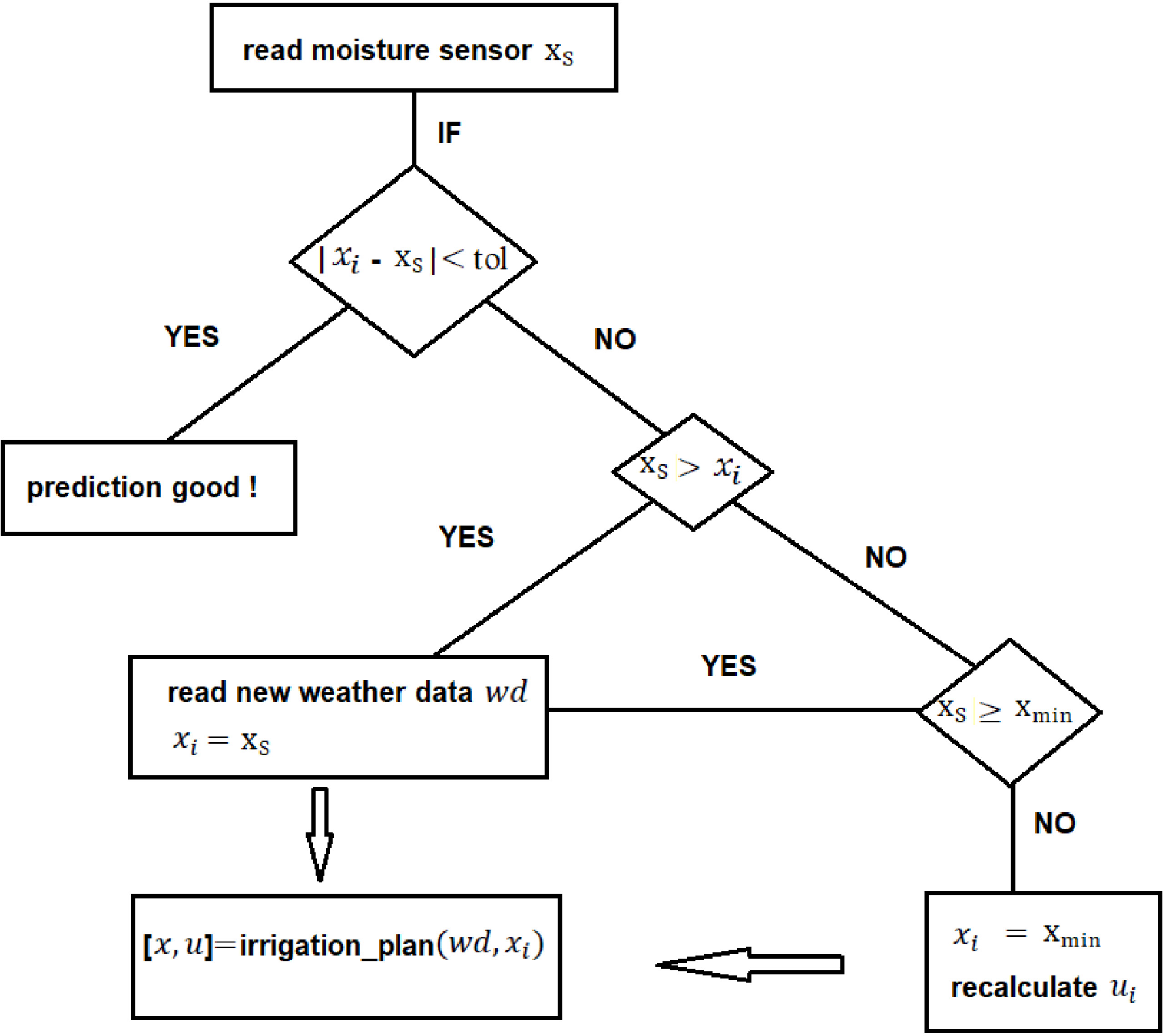
The replan algorithm detects if the soil moisture read by the sensor significantly differs from that predicted in the Irrigation plan for the current day. If that is the case, two situations may occur: the state constraint is not violated, and then the process is repeated with new data. If the state constraint is violated, it is necessary to calculate an irrigation value to avoid state constraint violation. New data are then considered imposing that the initial state is now x_min and the program is rerun. This approach is simpler and different from the one based on a penalty approach presented in [21].

So far, the model assumed that the whole field is described as one point in space. The irrigation plan for the whole crop field is designed for that point, implying that the spatial distribution of irrigation measures is uniform. A more realistic model would consider several irrigation points.

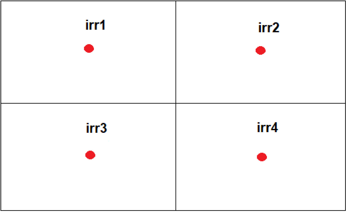
For simplification, the model assumes that the field is rectangular and consists of several smaller rectangular areas (example in Figure 2). An irrigation point at the center of each smaller rectangle receives an irrigation plan described in the previous sections. The new irrigation planning system can now cope with differentiated irrigation needs that depend on the spatial location.

Figure 2

Crop field with multiple irrigation points

The multiple irrigation points plan algorithm (detailed in the Appendix, part A2) is proposed and implemented to consider multiple irrigation points. After obtaining the irrigation plan for each irrigation point, the water redistribution algorithm will verify if each irrigation point can irrigate the necessary amount of water.

The multiple irrigation points plan algorithm uses the notation as follows: N is the number of irrigation points, ND is the number of days included in the irrigation planning, P(N; day) is the irrigation plan on a specific day (day=1,...ND) in each of the N irrigation points and C(N) is the maximum capacity of each irrigation point.

The algorithm verifies if all the irrigation points can fulfil the irrigation plan for that day. If, for instance, an irrigation point cannot fulfil its needs, the water redistribution algorithm seeks the possibility to fulfil the necessary needs in other irrigation points. This information is passed on to the farmer. Suppose it is impossible to fulfil every irrigation point's needs after fulfilling the irrigation needs at the points where that is possible. In that case, the available water is redistributed in the irrigation points where water is needed.

Since the information on the water deficits (wd) at each irrigation point has reached the farmer, eventually, he will be able to obtain water elsewhere and proceed with the multiple irrigation points plan.

Different scenarios were considered to validate the mathematical model qualitatively. Although the model assumes using daily data only, an hourly-based model will be used (providing the future the data is hourly), allowing us to have a more accurate model. The data used (weather and local moisture in the soil) to support the findings of this study are available from the corresponding author upon request.

In the following subsections, the replan algorithm and the multiple irrigation points plan algorithm will also be qualitatively validated using a set of scenarios.

Mathematical model validation

Several scenarios considered to validate the mathematical model are outlined below.

Base Scenario 1

This scenario considers the weather data, soil data, and crop data (read from a text file) describing a period when the rainfall was scarce. The weather data for those days (taken from a weather station placed on the crop field) are following:

Rainfall = [10 0 0 0 0 0 0 10 0 0] [mm]

WindSpeed = [2.8 3 2.4 2.4 3 2.2 2.7 2 2.2 2.8] [m/s]

MinTemp = [17.4 17.1 15.2 15.3 15.1 15.6 16.3 16.3 15.4 14.7] [°C]

MaxTemp = [24.4 20.8 23.1 22.2 24.9 26.9 29.3 23.6 19.4 20.4] [°C]

The crop under consideration is grass in the region of Oporto (NW of Portugal). The minimum amount of water in the soil is 18.72 mm. This Base Scenario 1 also assumes that the field is horizontal and all the excess water is lost (C_S = 1) if the amount of water in the soil is above the field capacity (the soil is saturated). Taking Base Scenario 1 into account, the OCP was written in AMPL [28] and solved by a primal-dual interior-point algorithm that uses filter line search method [29], known as IPOPT solver available in the NEOS platform. This method's local and global convergence properties were analyzed in [30]. The optimal solution obtained for irrigation and moisture in the soil is shown in Figure 3.

Figure 3

Base Scenario 1 results when rainfall is scarce

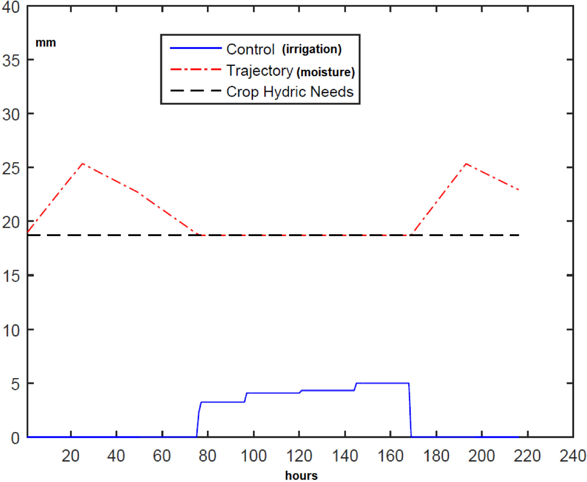
From Figure 3, it is possible to see that the irrigation is not necessary for the first three days and the last three days because it rained on the first and eighth days. The total consumption of water was 16.2 mm. The problem was solved in 0.12 s of CPU time.

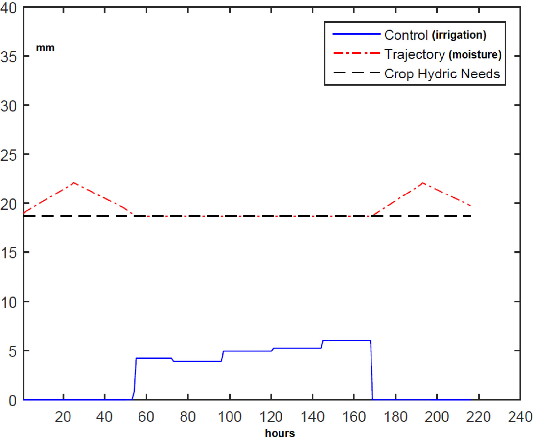
Scenario 1a is a modification of Base Scenario 1. Field inclination is changed to α=20°, and it is assumed that 50% of runoff is lost (R_F = 0.5), keeping all the other parameter values. The optimal solution of the problem for Base Scenario 1a is shown in Figure 4. Note that there is rain in that period, but runoff losses occur due to the field not being flat, making irrigation necessary. The water consumption is 23.3 mm. The irrigation starts earlier (compare Figure 3). When it rains, soil moisture is lower compared to Base Scenario 1.

Scenario 1b considers the data of Base Scenario 1 with the horizontal field again, but the maximum temperature on the fifth day is 38.9 °C instead of 24.9 °C. Figure 5 depicts the optimal solution for Scenario 1b. As it was much hotter on one of the days, evapotranspiration of the crop increased significantly, and so did the irrigation need. Compared with Base Scenario 1, the water consumption increased to 20.3 mm.

Figure 4

Scenario 1a: α=20° and R_F = 0.5

Figure 5

Scenario 1b: the maximum temperature on the fifth day is 38.9 °C instead of 24.9 °C

One could consider more variations of Base Scenario 1. However, from the above scenarios, it is possible to conclude that the model behaves well qualitatively. As one could expect, if there is a slope in the soil, the irrigation increases due to the runoff, and the same happens when the temperature is higher in periods of draught.

Base Scenario 2

This scenario considers the weather data, soil data, and crop data (read from a text file) for a regular rainfall period in April. The weather data for those days (taken from a weather station placed on the crop field) are following:

Rainfall = [5.8 4 13 7.1 4.8 0 0 0 50.3 3.8 3.0] [mm]

WindSpeed = [4.5 7.8 2.9 3.1 2.9 2.7 6.9 2.2 3.2 2.7] [m/s]

MinTemp = [12 14 11 10 9 8 14 15 15 15] [°C]

MaxTemp = [16.1 17.1 16.4 17.2 16.8 17.1 16.7 16.3 17.2 16.6] [°C]

Again, the crop considered was grass in the region of Oporto (NW of Portugal). The minimum amount of water in the soil is 18.72 mm. In the Base Scenario 2 is also considered that the field is horizontal $(\alpha =0^{\underset{\_}{\circ }})$ and all the excess water is lost (C_s = 1) if there exists saturation. The optimal solution of the OCP based on Scenario 2 is shown in Figure 6. Note that irrigation is not necessary because the soil moisture is always above x_min. Indeed the soil reaches the field capacity at a certain point, x > x_FC with x_FC = 46.8 mm. The total consumption of water was 0 mm. IPOPT solver took approximately 0.1 s CPU time to solve the problem.

Figure 6

Base Scenario 2 results when rainfall is regular

In Scenario 2a, the weather conditions are the same as in Scenario 2, but it is assumed that field has a slope of $\alpha ={20}^{\underset{\_}{\circ }}$, and 50% of runoff is lost (R_F = 0.5). The optimal solution of the problem for this scenario is shown in Figure 7. Interestingly, the amount of water lost by runoff is significant due to the field inclination and runoff loss coefficient. It can lead to a point where it might be necessary to irrigate, even for a period where plenty of rain fell. In such a scenario, one can conclude that building a tank to collect runoff would benefit the farmer.

Figure 7

Scenario 2a: α = 20° and R_F = 0.5

Replan Algorithm Validation

As base scenario to validate the replan algorithm, a very dry period was considered. The weather data for these days are the following:

Rainfall = [0 0 0 0 0 0 0 01.02 0] [mm]

WindSpeed = [2.8 3 2.4 2.4 3 2.2 2.7 2 2.2 2.8] [m/s]

MinTemp = [17.4 17.1 15.2 15.3 15.1 15.6 16.3 16.3 15.4 14.7] [°C]

MaxTemp = [24.4 20.8 23.1 22.2 24.9 26.9 29.3 23.6 19.4 20.4] [°C]

Figure 8

Replan base scenario - set of very dry days, and actual values for the necessary data are as expected

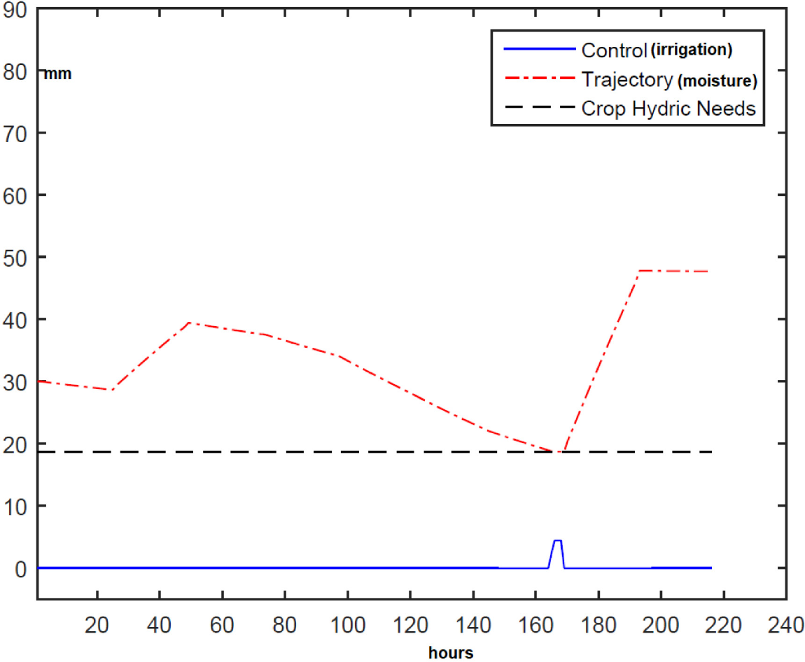
It is assumed the measured moisture in the soil (x_s) was close to the one predicted by the initial irrigation plan (trajectory) – no replan was needed. The optimal solution of the OCP for the replan base scenario is shown in Figure 8. The total water consumption was 33.35 mm. The real moisture in the soil was as follows:

x_s = [19 18.7 18.7 18.7 18.7 18.7 18.7 18.7 18.7 18.7] [mm]

Let us now assume that the moisture sensor measures a different value (lower) than expected on the fifth day:

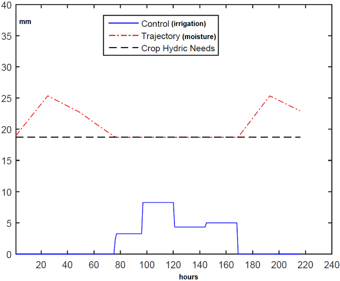
x_s = [19 18.7 18.7 18.7 15 18.7 18.7 18.7 18.7 18.7] [mm]

Replan will be activated. Figure 9 depicts the optimal solution of the OCP for this scenario. The hydric needs are the needs of the crop. It is essential to satisfy this constraint. In the case of constraint violation (x_s < x_min), it is imperative to correct the needs of the water to avoid crop damage/failure – using the second part of the replan algorithm described before.

As shown in Figure 9, in the first four days the initial planning solution (solution IS: control IS and trajectory IS) is equal to the solution obtained in the replanning (solution R: Control R and Trajectory R). After that, the water needs exceed the planning solution on the fifth day. In this scenario, the amount of water used by the irrigation systems was 36.4 mm.

Figure 9

Replan base scenario with real moisture value on the fifth day lower than expected [31]

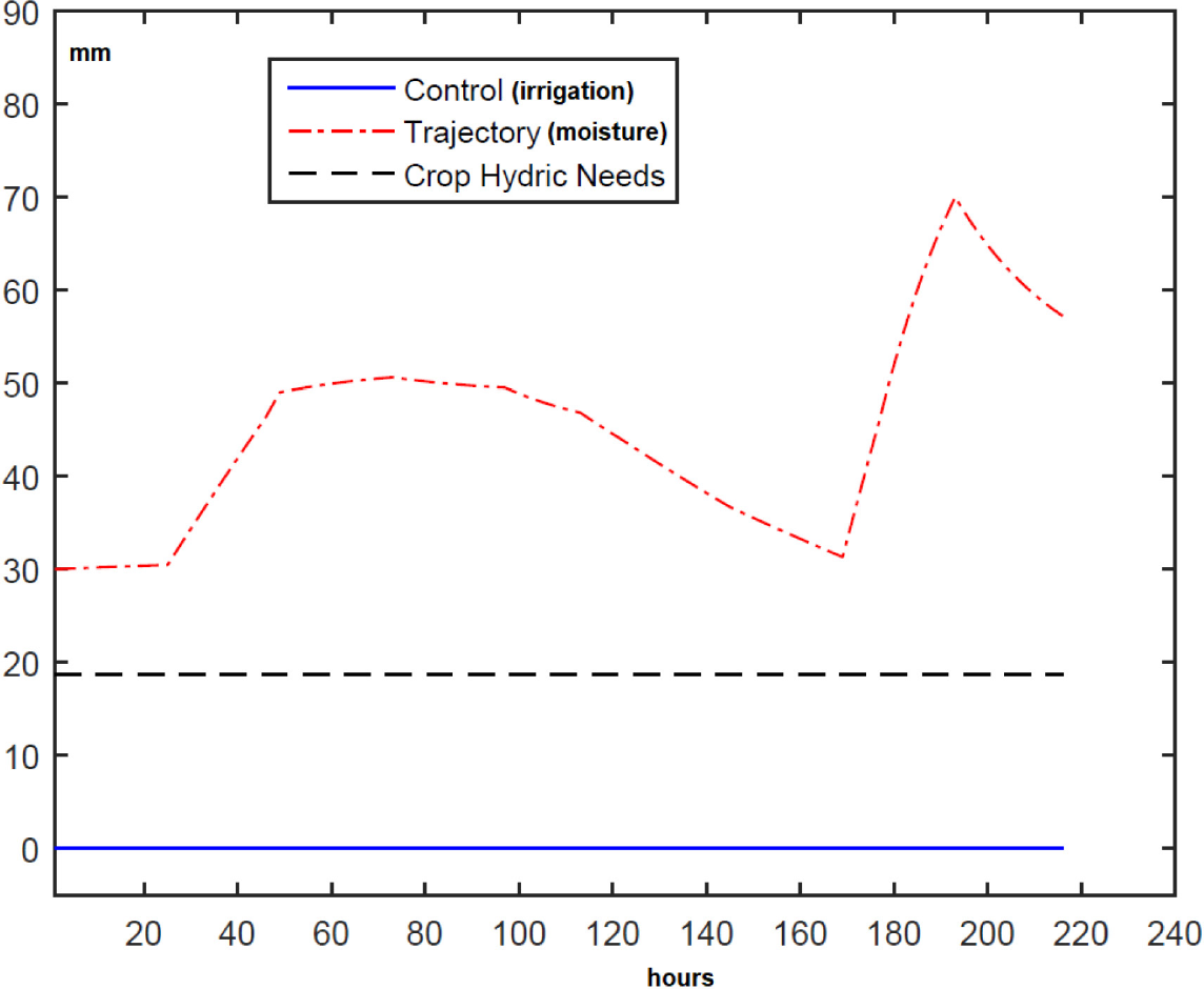
Next, another similar example is shown to justify using the replan and its qualitative validation. Let us now assume that the moisture sensor measures a different (higher) value than expected in the fifth day:

x_s = [19 18.7 18.7 18.7 22 18.7 18.7 18.7 18.7 18.7] [mm]

Figure 10

Replan base scenario with real moisture value on the fifth day higher than expected [31]

Results can be seen in Figure 10. As expected, the irrigation on the fifth day decreased. In this scenario, the amount of water used by the irrigation systems was 29.9 mm.

From the above scenarios and their results, it is possible to conclude that the replan strategy is a vital tool in designing smart irrigation systems, enabling to detect deviations from an ongoing prediction and acting accordingly. It allows to save water and keeps the crops safe.

This article proposed to design an improved mathematical model based on the one presented in the authors' previous publications. The model allows having a smart irrigation system, provided that the irrigation requirements are feasible for given data. (Note that in the authors' publications [21] and [22], the solution for a similar problem was numerically validated, taking into account theoretical developments in Optimal Control, namely the Maximum Principle). New features of the model include the slope of the soil, the possibility to include a percentage of water losses due to runoff, and a percentage of water losses if the soil is at field capacity. A qualitative study shows that the improved model can address these features.

If the moisture sensors detect a value much different from the expected by the irrigation plan, a replan strategy is applied to obtain a new irrigation plan. The proposed model incorporates a new constraint to impose that the soil moisture does not violate the state constraint, which forces to add to the control variable the value needed. Several examples were given to validate the mathematical models proposed in this manuscript qualitatively.

The model is essential since it is not uncommon that weather forecasts are wrong, and therefore, the forecasted value of the soil moisture is wrong. Therefore, by introducing replan, it is possible to save water and, at the same time, guarantee crop safety.

The article also proposed a new approach to deal with multiple irrigation points. Despite its simplicity, it allows redistributing the available water if an irrigation point cannot provide all needed according to its irrigation plan. Once again, in draught periods, this is an essential improvement since it is possible that an irrigation point cannot fulfil its duty, and neighbouring irrigation points might help.

From the results shown in this manuscript, the authors believe that they have developed a valuable tool to use in a farm field and hopefully help to achieve better and more sustainable agriculture. In the future, on-site tests are planned, namely, model calibration to obtain a reliable smart irrigation software prototype. Additional moisture sensors and local weather data are to be acquired and considered inputs to the mathematical model presented in this paper.

The research presented here is integrated with a research project funded by several national and international entities mentioned in the Funding Statement. It aims to design, create, and install a smart irrigation prototype on a farm field in the North of Portugal.